Suppose we have 2 datasets containing the Product Name, Quantity, and Sales amount of 2 shops in different worksheets.
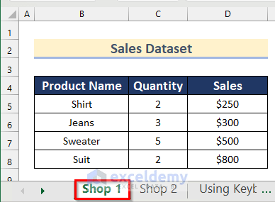
The above image is the dataset for Shop 1.
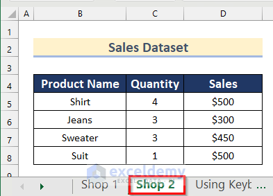
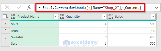
And above is the Shop 2 worksheet, which contains information about the other shop.
Using these 2 worksheets we will demonstrate how to create a table from multiple sheets in Excel using various methods.
Method 1 – Using Keyboard Shortcut
We can use the “Alt + D” keyboard shortcut to open the PivotTable and PivotChart Wizard to create a table from multiple sheets. This will sum the values in the 2 sheets and give us a summary for the 2 shops.
Steps:
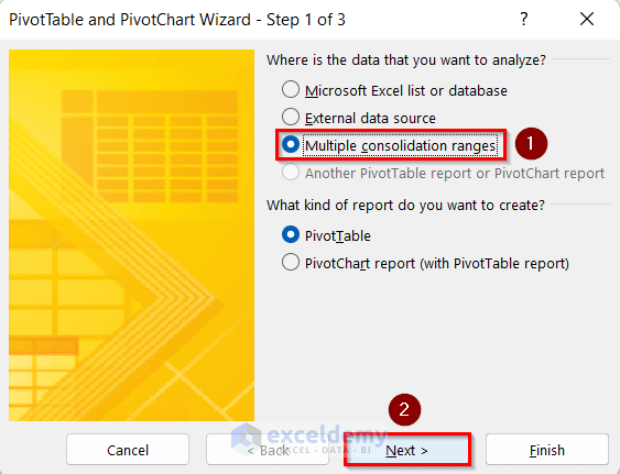
- Press Alt + D and then press P.
The PivotTable and PivotChart Wizard box opens.
- Select the Multiple consolidation ranges option.
- Click on OK.
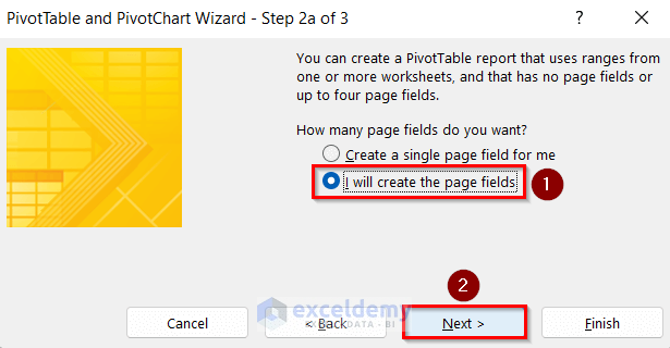
- Select the I will create the page fields option.
- Click on Next.
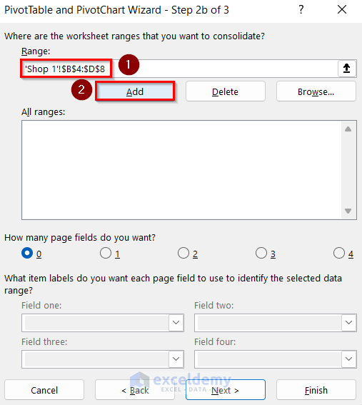
- Select the range B4:D8 from the Shop 1 worksheet as the Range to consolidate.
- Click on Add.
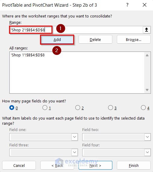
- Select the range B4:D8 from the Shop 2 worksheet as the Range to consolidate.
- Click on Add.
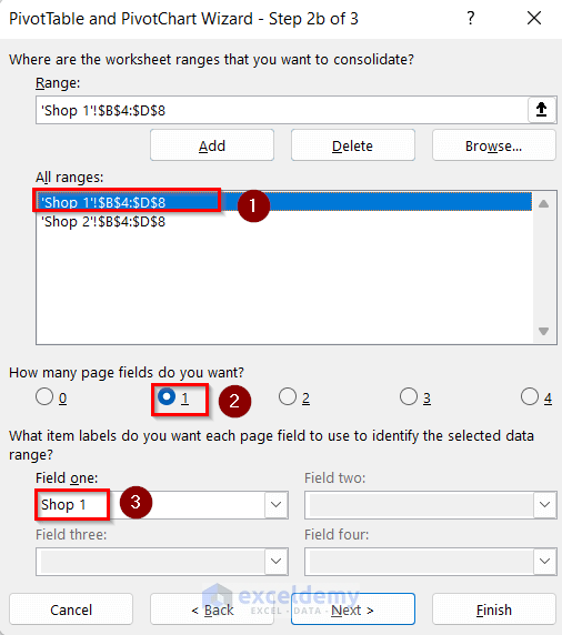
- Select the range from the Shop 1 worksheet and set 1 as the page fields number.
- Enter Shop 1 in the Field one box.
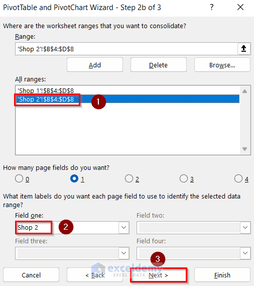
- Select the range from the Shop 2 worksheet and enter Shop 2 in the Field one box.
- Click on Next.
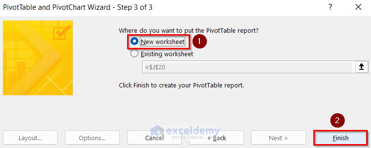
- Select the New worksheet option as the destination to put the PivotTable report.
- Click on Finish.
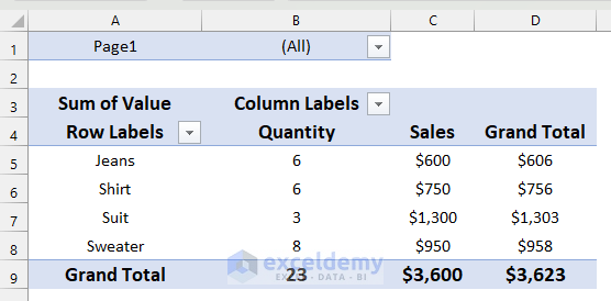
A pivot table is created using the datasets from both sheets.
Read More: How to Create Table from Another Table in Excel
Method 2 – Using Relationships Feature
Suppose we have datasets in multiple sheets which do not contain the same fields, and we want to summarize that information in one table. We can use the Relationship Feature for this purpose.
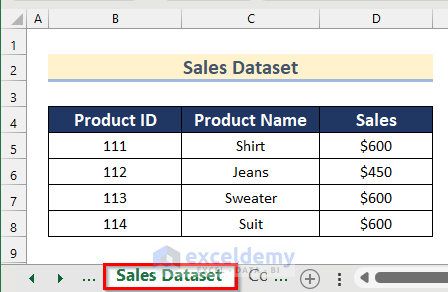
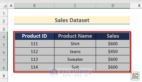
Here, we have a dataset containing the Product ID, Name and Sales of a shop in the Sales Dataset worksheet.
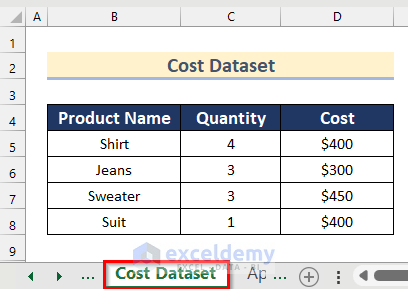
Additionally, in the Cost Dataset worksheet, we have information about the Product Name, Quantity and Cost of making those products.
Let’s create a table using these 2 worksheets which contain different fields.
Step 1 – Creating Tables
First we create tables in the individual worksheets to create a relationship between them.
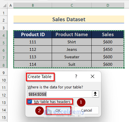
- Select the range B4:D8 from the Sales Dataset worksheet.
- Press Ctrl + T to create a table.
The Create Table box will pop up, showing that the cell range has already been selected.
- Mark the My table has headers option.
- Click on OK.
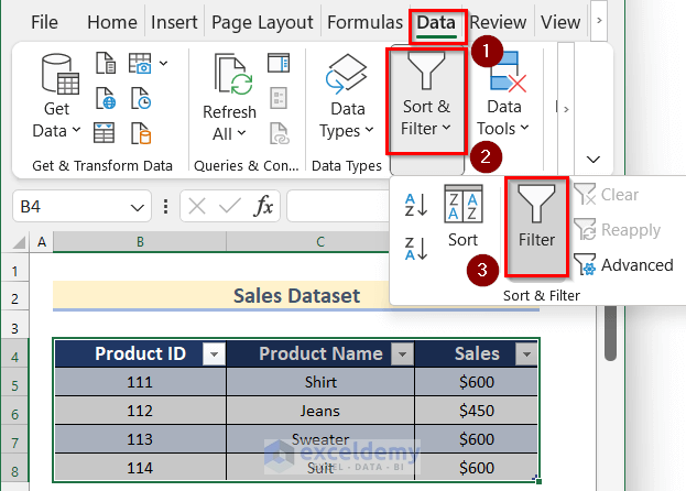
- To remove the filters from the table, go to the Data tab.
- Click on Sort & Filter >> Filter.
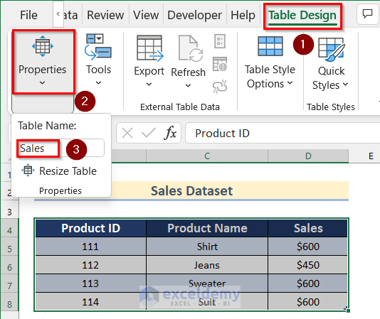
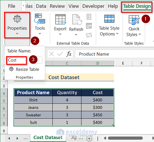
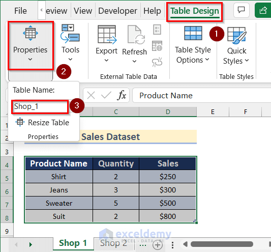
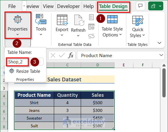
- To set a name for the table, go to the Table Design tab.
- Click on Properties.
- Enter Sales in the Table Name box.
- Similarly, we’ll create a table using the dataset in the Cost Dataset worksheet and remove filters from the fields.
- Go to the Table Design tab.
- Click on Properties.
- Enter Cost in the Table Name box.
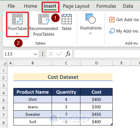
Step 2 – Inserting Pivot Table
- In the Cost Dataset worksheet, go to the Insert tab.
- Click on PivotTable.
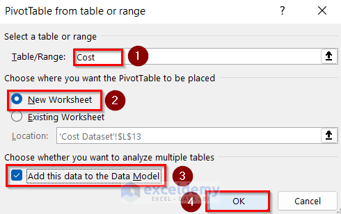
The PivotTable from table or range box will open.
- Enter Cost in the Table/Range box.
- Select the New Worksheet option.
- Mark the Add this data to the Data Model option.
- Cick on OK.
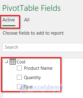
Another worksheet opens with the Cost table as the Active table.
Step 3 – Using Relationships Feature
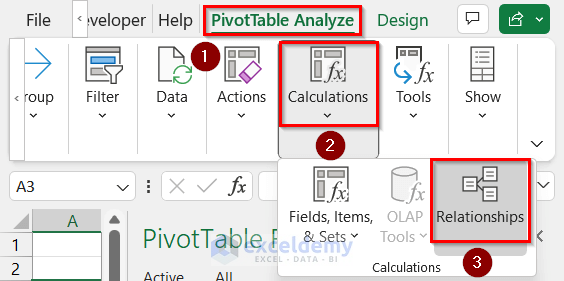
- Go to the PivotTable Analyze tab.
- Click on Calculations.
- Click on Relationships.
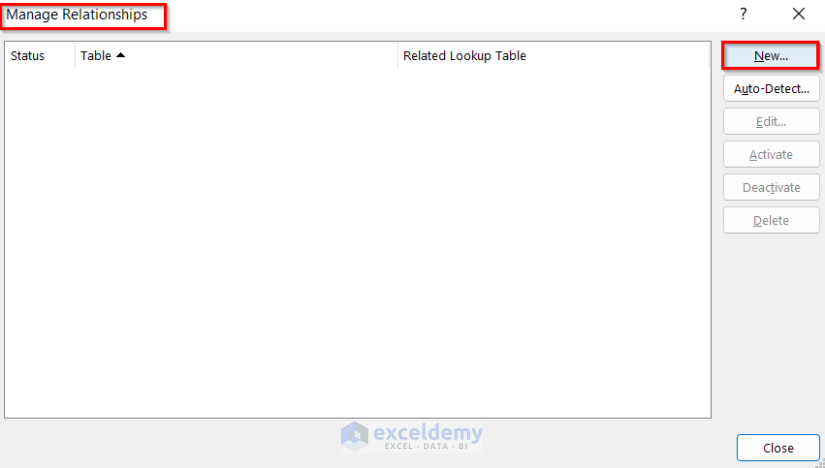
The Manage Relationships box will appear.
- Click on New.
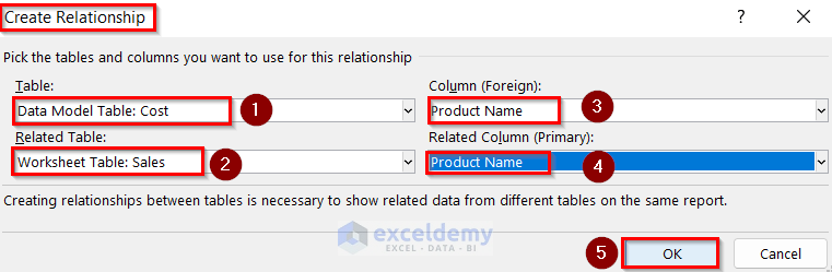
The Create Relationship box will open.
- Select Cost as the Table, Sales as the Related Table, Product Name as the Column (Foreign), and Product Name as the Related Column (Primary).
- Click on OK.
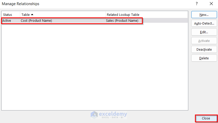
A relationship is created between the two tables.
- Click on Close.
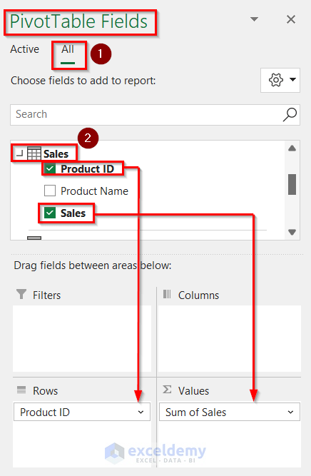
- In the PivotTable Fields toolbox, go to the All option.
- Click on Sales to expand the field names.
- Drag the Product ID field into Rows, and Sales into Values.
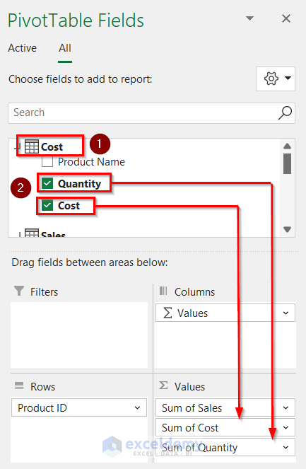
- Click on Cost to expand the field names.
- Drag the Quantity and Cost fields into the Values box.
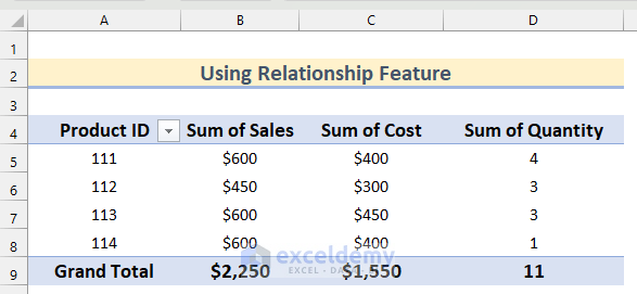
- A table is created using datasets from multiple sheets.
Read More: How to Mirror Table on Another Sheet in Excel
Method 3 – Using Get Data Feature
Steps:
- Create a table using the cell range B4:D4 from Shop 1 worksheet by applying the steps in Method 2.
- Go to the Table Design tab.
- Click on Properties.
- Enter Shop_1 in the Table Name box.
- Similarly, create a table using the cell range B4:D4 from the Shop_2 worksheet and set the table name as Shop 2.
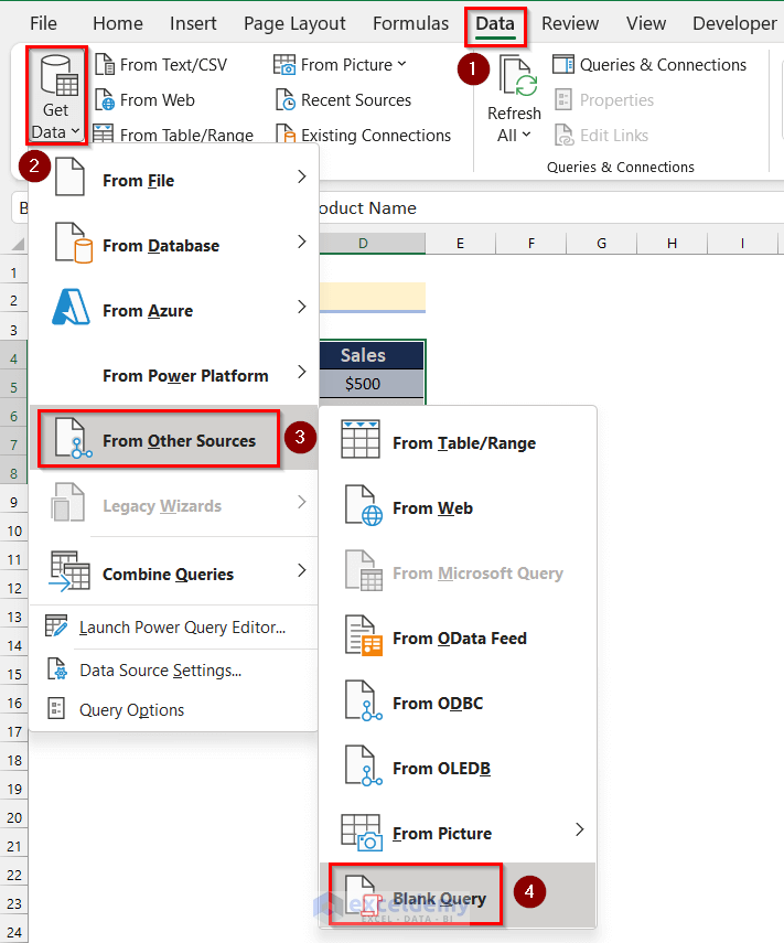
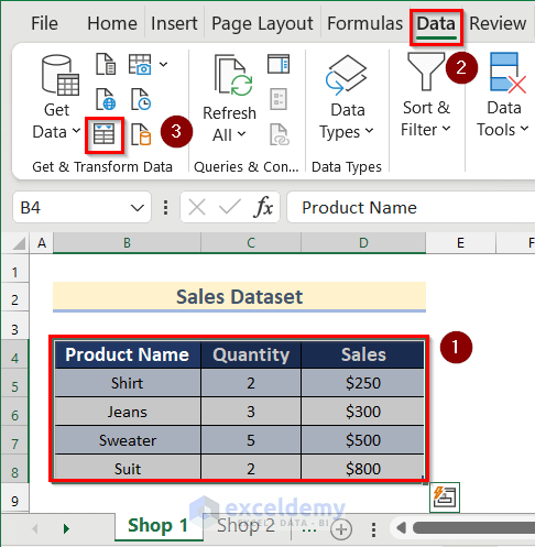
- Go to the Data tab.
- Click on Get Data.
- Click on From Other Sources.
- Select Blank Query.
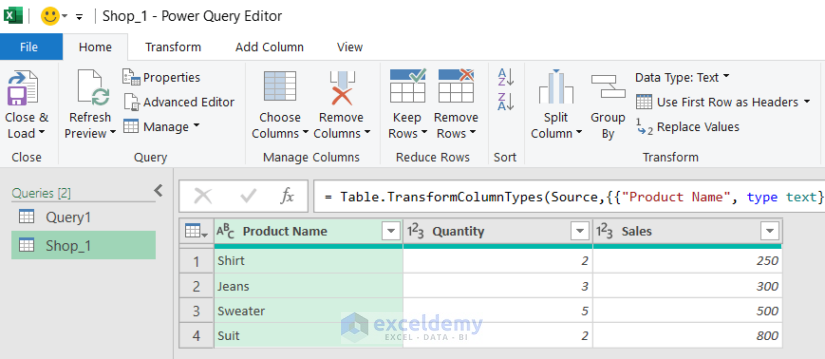
A blank query will open in the Power Query Editor box.
- Enter the following formula in the formula box and press Enter:
= Excel.CurrentWorkbook()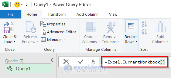
- All the Tables will be loaded in the current workbook.
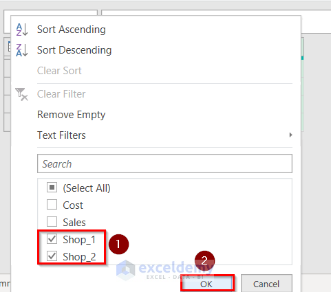
- To select the preferred tables, click on the button shown below.
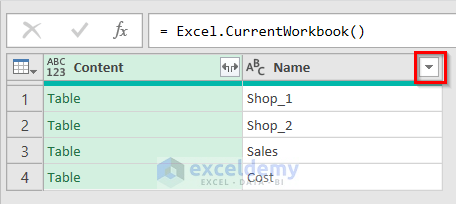
- Select only the Shop_1 and Shop_2 tables.
- Click on OK.
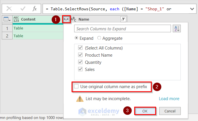
- Click on the button shown below.
- Uncheck the Use original column name as prefix option.
- Click on OK.
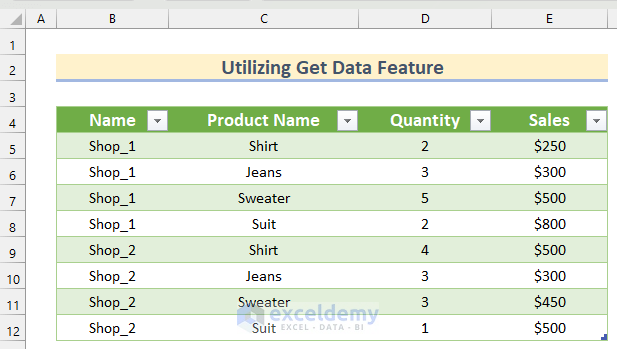
All the data from the 2 tables will be loaded together in a table, and a new column will be added containing the Name of the Shops.
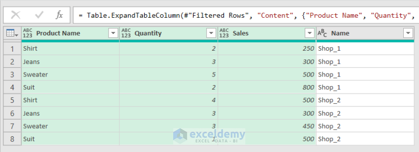
- If you want, you can drag the Name column to make it the leftmost column.

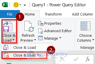
- Click on Close & Load.
- Select Close & load To.
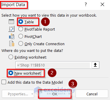
The Import Data box will open.
- Select the Table option.
- Select the New worksheet option as the destination for the table.
- Click on OK.
- Our table is created.
Read More: How to Create Table from Another Table with Criteria in Excel
Method 4. Using Append Queries in a Pivot Table
Step 1 – Creating Connection
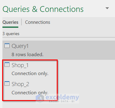
First we need to create a connection between the 2 tables in the different sheets.
- Create Shop_1 and Shop_ 2 tables by going through the steps in Method 3.
- Select the Shop_1 table.
- Go to the Data tab.
- Click on Form Table/Range.
The Shop_1 table will open in the Power Query Editor.
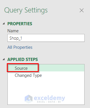
- Select Source from the Applied Steps box.
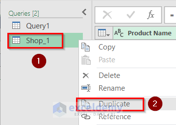
- Select the Shop_1 table and right-click on it.
- Click on Duplicate.
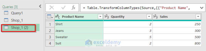
A duplicate table of Shop_1 named Shop_1(2) will be created.
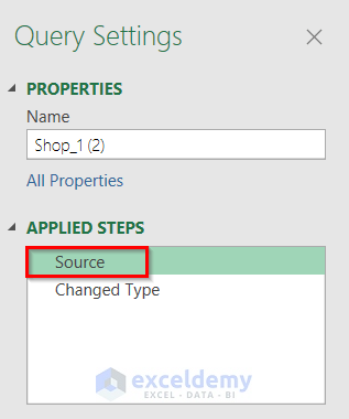
- Select this table and click on Source from the Applied Steps box.
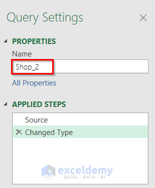
- Change the Name to Shop_2 in the formula box.
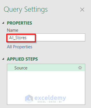
- Type Shop_2 as Name in the Query Settings.
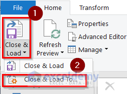
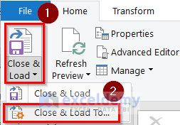
- Click on Close & Load.
- Click on Close & Load To.
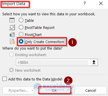
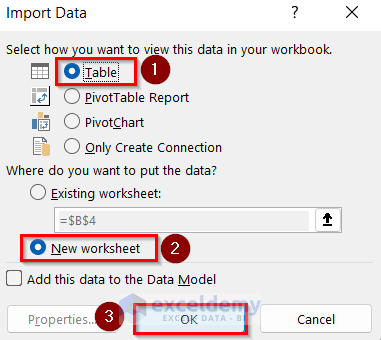
The Import Data box will open.
- Mark the Only Create Connection option.
- Click on OK.
A connection is created between these 2 tables.
Step 2 – Using Append Queries Feature
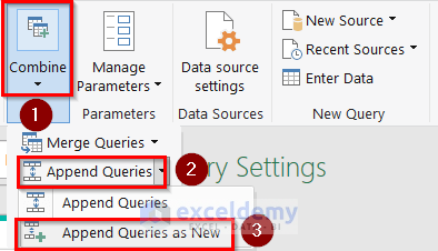
Now we can use the Append Queries feature to append data from the two tables.
- Click on either of the 2 tables in the Queries and Connections toolbox to open the Power Query Editor again.
- Click on Combine.
- Click on Append Queries.
- Click on Append Queries as New.
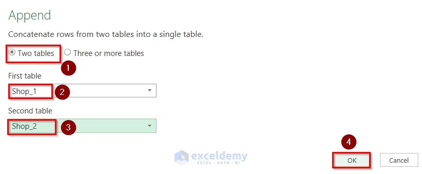
The Append box will appear.
- Select the Two tables option.
- Select Shop_1 as the First table and Shop_2 as the Second table.
- Click on OK.
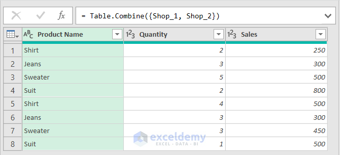
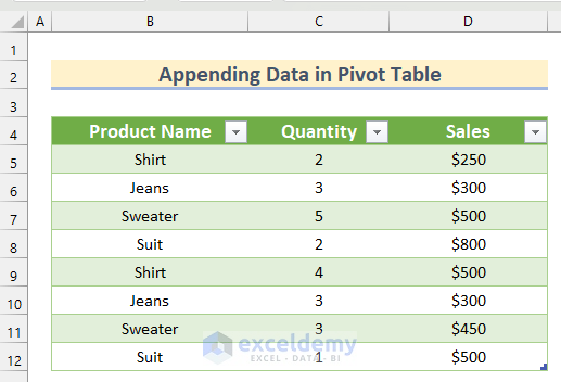
The data from the two tables will be appended together.
- Set All_Stores as the Query Name.
- Click on Close & Load.
- Click on Close & Load To.
- In the Import Data box, select the Table option.
- Select the New worksheet option.
- Click on OK.
- A table is created by appending data from multiple sheets.
Read More: How to Create a Lookup Table in Excel
Download Practice Workbook
Related Articles
- How to Make 3D Table in Excel
- How to Make a Decision Table in Excel
- How to Create a League Table in Excel
- How to Make a Table Bigger in Excel
<< Go Back to Excel Table | Learn Excel
Get FREE Advanced Excel Exercises with Solutions!
