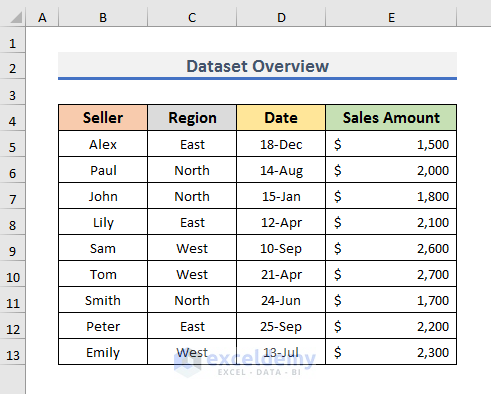
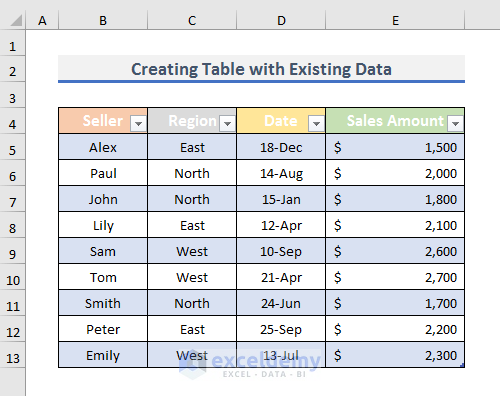
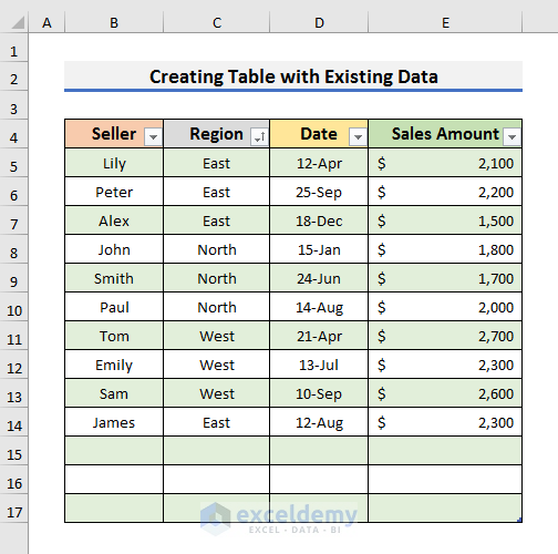
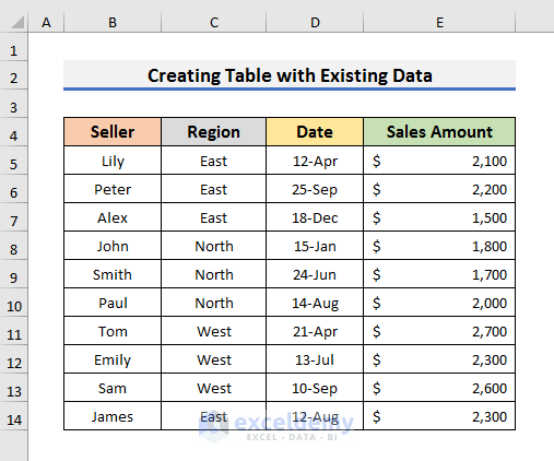
We will use a dataset containing information about some Sellers’ Sales Amounts. It also includes the Region and Dates of the sales.
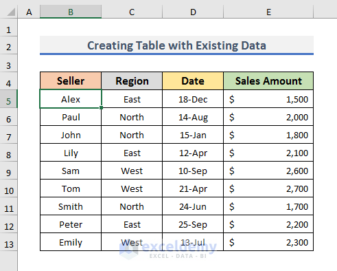
STEP 1 – Create a Table with Existing Data
- Select any cell of the existing dataset.
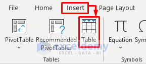
- Go to the Insert tab and click on the Table option.
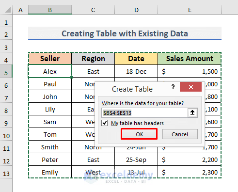
- A Create Table dialog box will appear.
- It will show the data range for the table. If you do not want the whole data in your table, select the range you want to insert inside the table. In our case, the range is B4:E13.
- Check the ‘My table has headers’ option if the table contains headers. Otherwise, uncheck it.
- Click OK to move forward.
- The existing data will convert into a table.
Read More: Create Table in Excel Using Shortcut
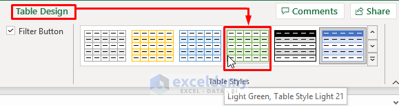
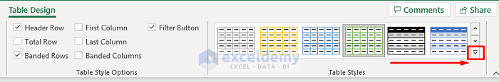
STEP 2 – Change the Table Design
- Select a cell in your table to make the Table Design tab appear in the ribbon.
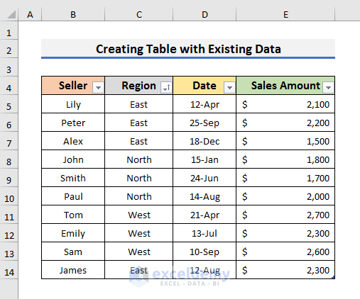
- Navigate to the Table Design tab and select a style from the Table Styles section.
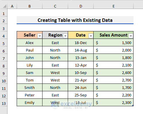
- Here’s a sample.
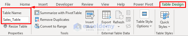
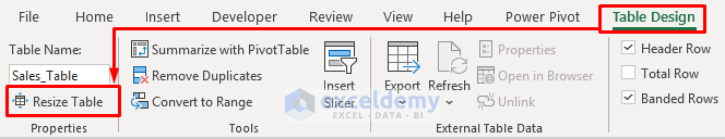
STEP 3 – Name the Excel Table
- Go to the Table Design tab and type the name inside the ‘Table Name’ box.
- You can’t use a space.
- Hit Enter to set the name.
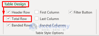
STEP 4 – Insert the Total Row
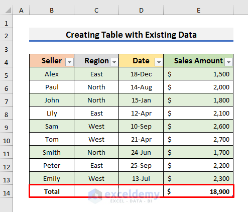
- Go to the Table Design tab and check the Total Row option.
- You will see the sum of the sales amount in the last row of the table.
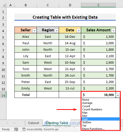
- If you click on Cell E14, a drop-down menu will appear.
- You can select different types of functions from there to see the Average, Count, Max, Min, Variance, and many more values of the sales amount.
Read More: How to Create a Table Without Data in Excel
STEP 5 – Sort the Excel Table
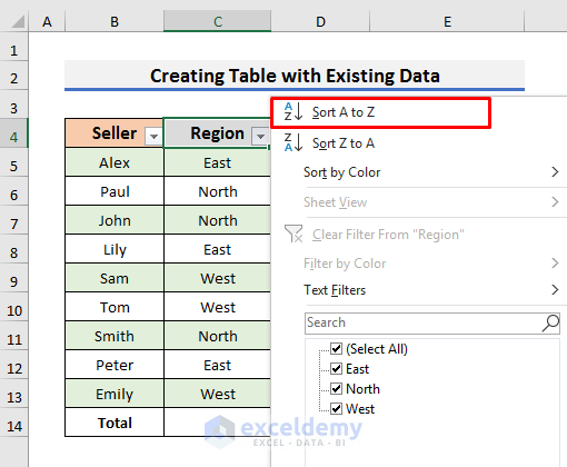
- Click on the drop-down arrow in a header.
- Select Sort A to Z from the menu. It will sort the dataset in ascending alphabetical order.
- You can also sort it in descending order by selecting the Sort Z to A option.
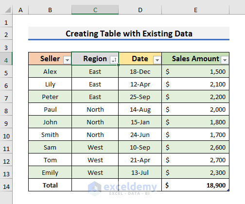
- After sorting, the table will look like the picture below.
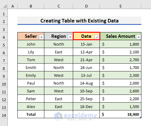
- You can also sort the table from the oldest to the newest dates.
Read More: How to Create a Table with Subcategories in Excel
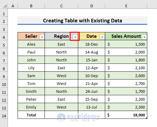
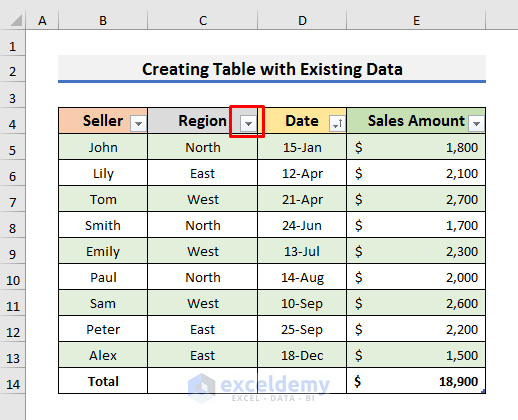
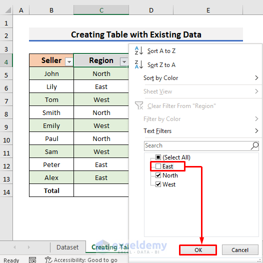
STEP 6 – Filter the Table in Excel
- Click on the drop-down arrow of a header.
- We will filter the table using the Region. So, we clicked on the drop-down arrow of the Region header.
- We want to see the information about the sales of the North and West regions. We unchecked the East option.
- Click OK to proceed.
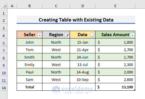
- The filter will be applied. You will see the sales amount of the North and West region only.
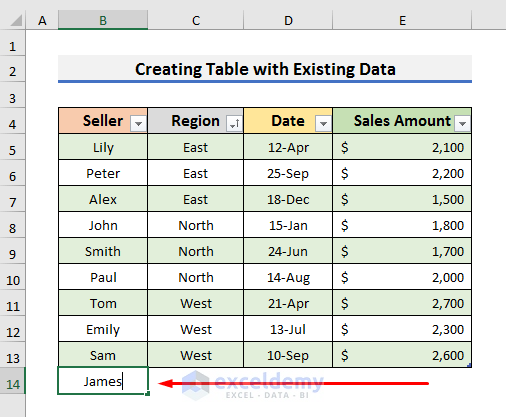
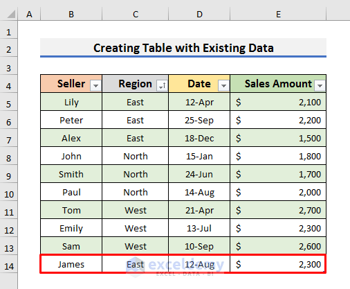
STEP 7 – Add New Data to the Table
- Move to the row below the last row and start typing your information. We have selected Cell B14 and typed James.
- Press Enter and the information will be added to the table.
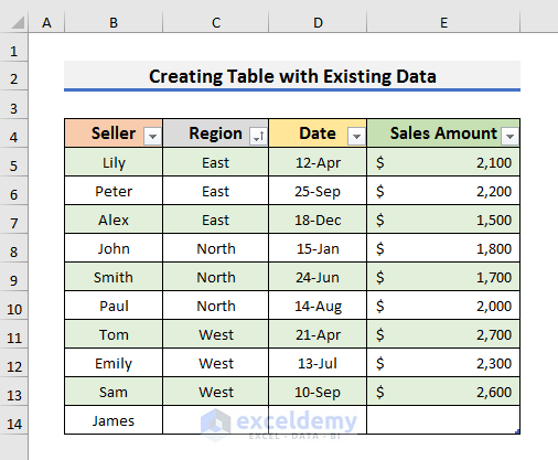
- Complete inserting all the data.
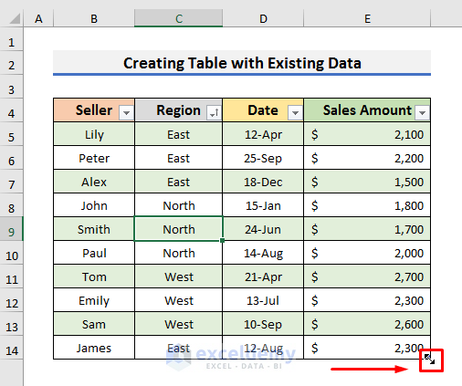
STEP 8 – Resize the Table
- Put the cursor on the bottom right corner of the last cell of the table.
- The cursor will change into a double-headed arrow.
- You can move it to increase the size of the table.
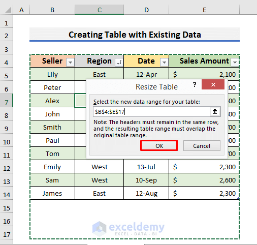
- Alternatively, you can go to the Table Design tab and select Resize Table.
- Change the range of the table to resize it.
- Our new range is B4:E17.
- Click OK in the Resize Table dialog box.
Final Output
How to Convert the Table to a Range in Excel
STEPS:
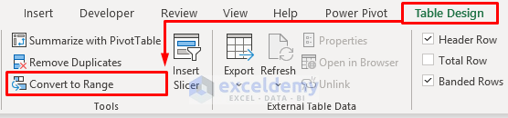
- Go to the Table Design tab and click on the More icon in the Table Styles section.
- Select None from the table styles.
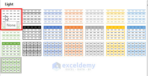
- The table will have no formatting.
- Go to the Table Design tab again and select the Convert to Range option.
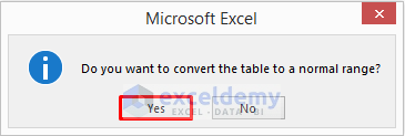
- A message will pop up.
- Click on Yes to move forward.
- The table will convert to a range like the existing dataset.
Read More: Create a Table in Excel Based on Cell Value
Download the Practice Book
Related Articles
- How to Create a Table with Merged Cells in Excel
- How to Create a Table in Excel with Multiple Columns
- How to Make a Table in Excel with Lines
- How to Add New Row Automatically in an Excel Table
<< Go Back to Excel Table | Learn Excel
Get FREE Advanced Excel Exercises with Solutions!
