How to Convert Range to Table in Excel (4 Methods)

To convert range to table in Excel:

Select a cell within your data range.
Press Ctrl+T.
In the Create Table box, tick the box “My Table has Headers” if the data contains headers.
Press OK.

Excel will convert the selected range to a table.

Converting a range to a table in Excel means transforming a selected group of cells, typically containing data, into an Excel Table. By converting ranges into tables, you can organize, manage, update, and analyze the entries in your dataset more efficiently.

In this Excel tutorial, you will learn how to convert the range to tables using Excel’s features and VBA macro code.

The following figure shows a dataset of Product Sales of multiple Products for different months, which is converted to a table in Excel using the table feature.

What Are Range and Table?

Range: In Excel, a group of selected cells in a dataset is range. You can select any number of cells in a dataset; the reference of the top leftmost and bottom rightmost cells is range. For Example, if we select cells (B4 to D13), then B4:D13 is the range in the dataset.

Table: Table is a kind of advanced range having inbuilt features. Excel Table works as a pre-structured up-to-date range with various offered features such as Header Rows, Total Rows, Banded Rows, First Column, Last Column, Banded Columns, Filter Button, etc.

It is very easy to distinguish Tables from Ranges. Excel Table has frozen heading, borderlines, auto-filter, and sort options as well as a distinct viewing format similar to the image below.

Why Convert Range to Table in Excel?

Here are some reasons to convert range to table:

Automatic filtering controls in table headers.
Quick and efficient sorting of data.
Easy data entry for dynamic chart and PivotTable updates.
Extends formatting and fills formulas automatically.
Automatic formula application across entire columns reduces errors.
Easy navigation through large datasets as Table headers remain visible.
Table Styles group provides swift and diverse formatting options.
Names appear automatically, contributing to a more organized spreadsheet.
Total Row enables efficient calculation of totals and summary statistics.

4 Ways to Convert Range to Table in Excel

In Excel, you can convert the range to table using Excel’s Table feature, Format as Table option, Pivot Table feature, and VBA macro.

Here are 4 ways to convert range to table in Excel:

Using Table Feature

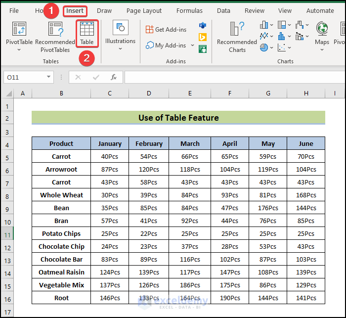
You can convert a range to a table by creating a table from a selected range using the Table feature of Excel.

To convert range to table using Table feature, follow the steps below:

Select a cell within your data range.
Go to Insert Tab> Tables group > Table. Or, press Ctrl+T.
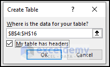
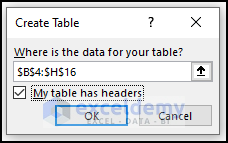
In the appeared Create Table box:
- Adjust the automatically selected range if needed.
- Tick the box My Table has Headers if the data range contains headers.
- Click OK.

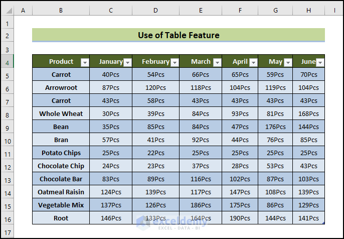
You can see the whole range converted into a table like the image below.

Using Format as Table Feature

Excel’s Format as Table feature quickly converts a range of cells to a table with its own style.

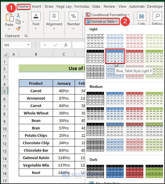
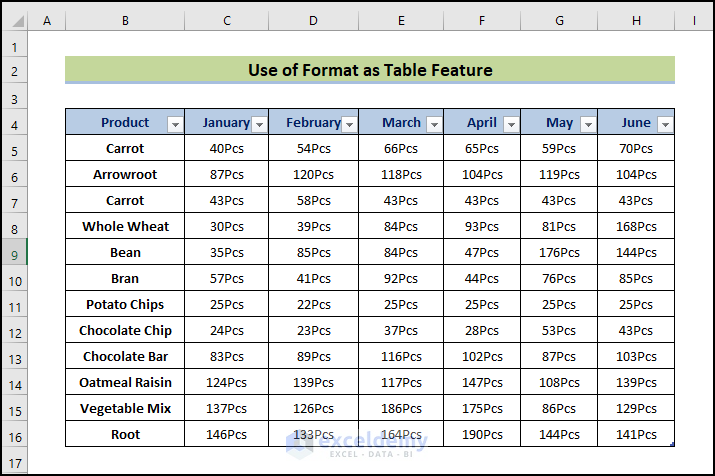
Follow the steps below to convert the range using Format as Table feature:

Select the range to convert.
Go to the Home Tab and select Format as Table from the Styles section.
Choose any of the Styles to format the range as a table.
In the Create Table window:
- Check the range.
- Tick the “My table has headers box“.
- Click OK.

Finally, the specified range will be converted into a table.

Using Pivot Table Feature

You can also convert range by inserting a special kind of table, which is Pivot Table. The Pivot Table is handy for displaying a range in the desired structure. Moreover, you can edit and arrange rows and columns and paste the table into a new worksheet according to your needs using a pivot table.

To use Pivot Table to convert range to table, go through the steps below:

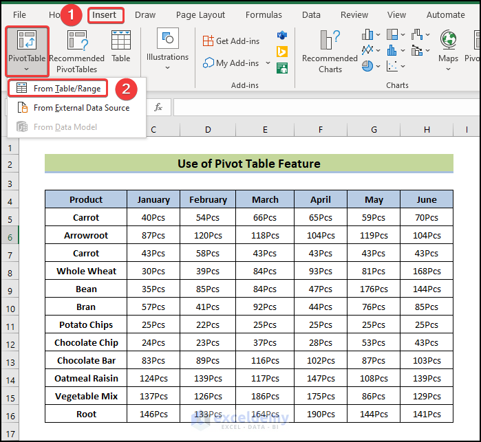
Select any cell in the data range.
Go to Insert tab > Tables section > Pivot Table > select From Table/Range.
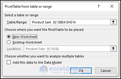
In the PivotTable from table or range box:
- Adjust the automatically selected cell range.
- Choose Existing Worksheet and select a Location to place the table if you do not want it to be placed in a new worksheet. Otherwise, keep New Worksheet option selected.
- Click OK.
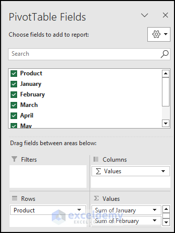
In the PivotTable Fields:
- Tick what column entries you want to display.
- Drag the column entries in any fields Filters, Columns, Rows, and Values.

Finally, the pivot table looks like the image below.

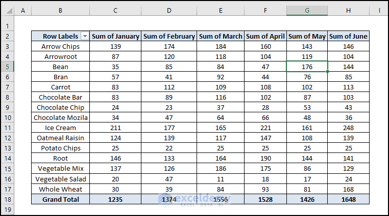
Note: You can see that PivotTable arranges the data alphabetically and shows the Sum of the values automatically.

Read More: Navigating Excel Table

Using VBA Macro

You can automate the conversion process from range to table using a VBA code.

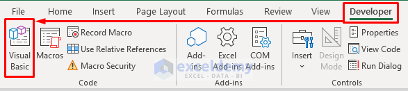
Follow the steps below to convert the range using the VBA macro:

Go to Developer tab > Code group > Visual Basic. Or press ALT+F11.
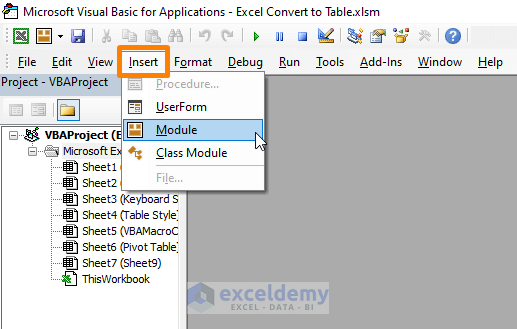
In the VBA window, click on Insert > select Module.

Paste the below VBA macro code inside the Module.

Sub ConvertRangetoTable()
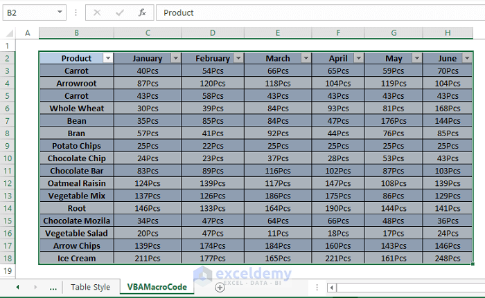
ActiveWorkbook.Sheets("VBAMacroCode").ListObjects.Add(xlSrcRange, Range("$B$2:$H$18"), , xlYes).Name = "Product_Sale"
End Sub

Press F5 to run the VBA macro code.

Lastly, go back to the worksheet and you will see the range converted into a Table like the following picture.

Read More: How to Make Excel Tables Look Good

Download Practice Workbook

Convert to Table.xlsm

Conclusion

In the article, you learned 4 different methods to convert a range into a table. You can use Table, Format as Table, PivotTable features, and VBA macro code to convert range to table according to your dataset. Please ask in the comment section below if you have any suggestions or queries.

Frequently Asked Questions

How do you convert an Excel table back to a regular range?

To convert an Excel table to a regular range:

Click anywhere in the table.
Go to the Table Tools Design tab > Tools section > select Convert to Range.

Are Excel tables compatible with older Excel versions?

Excel tables are available in newer versions (Excel 2007 and later). Some features may not be available in older versions, but basic functionality, such as sorting and filtering, remains compatible.

Can I customize the appearance of an Excel table?

You can customize the appearance of a table by using the various table styles available under the Table Tools Design tab, which includes options for banded rows, columns, and more.