How to Create a Table Array in Excel (3 Methods)

In this article, we will provide 3 useful examples of how to create and use a table array.

What Is Table Array in Excel

When we use a VLOOKUP or HLOOKUP function, we enter a range of cells in which to look up the required value, for example B5:C7 in the dataset below. This range is called the table_array argument.

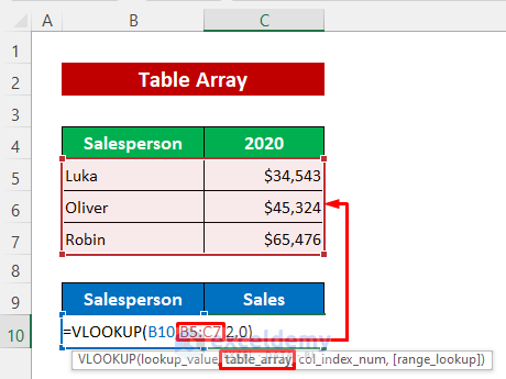
In the above image, the VLOOKUP function searches for a match of the value in B10 within the range B5:C7. B5:C7 is the table array argument here.

Create a Table Array in Excel: 3 Examples

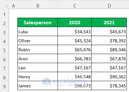
To demonstrate the examples, we’ll use the following dataset that represents some salespersons’ sales in two consecutive years.

Example 1 – Create a Table Array for VLOOKUP Function

First we’ll create a table array with a single table for the VLOOKUP function.

Steps:

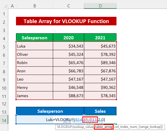
• Enter the following formula in Cell D14:

• Press Enter.

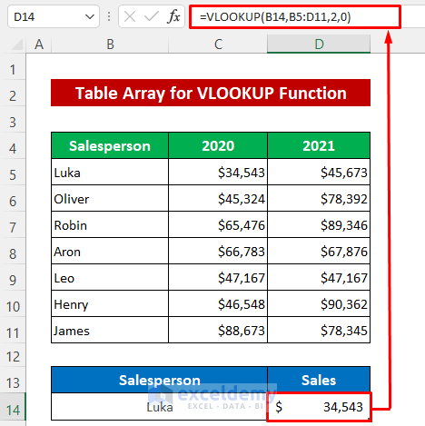
The lookup range B5:D11 is the table array argument.

Read More: Types of Tables in Excel: A Complete Overview

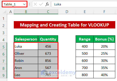
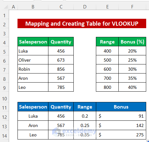
Example 2 – Mapping and Creating Table for VLOOKUP Function

Now we’ll create multiple table arrays for use with the VLOOKUP function. To illustrate, the dataset has been modified so that the first table shows the salespersons’ sold quantity and the second table represents the bonus percentage according to quantity range. First, we’ll set the named range for each table.

Steps:

• Select the data from the first table.
• Type a name for the selected range in the cell reference box and press Enter.

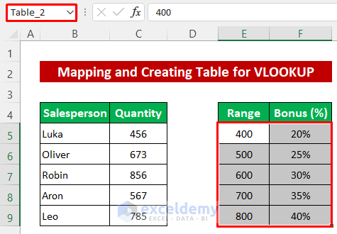
• Repeat the procedure to set a name for the second table.

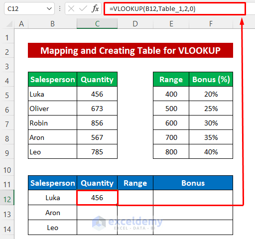
Now we’ll look up the quantity, range, and bonus for a particular salesperson.

• In cell C12, enter the following formula:

• Press Enter to return the quantity for Luka.

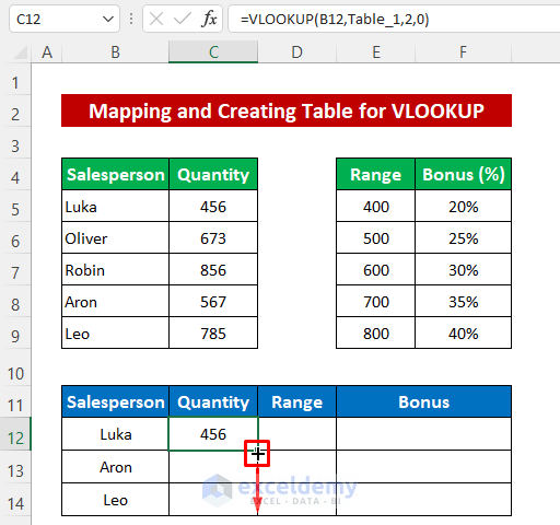
• Drag down the Fill Handle icon to copy the formula for Aron and Leo.

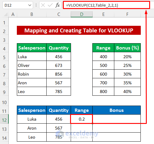
Now we’ll find the bonus percentage according to the quantity range. As the quantity is not exact in the range, we use the Approximate Match option in the VLOOKUP function by setting 1 as the fourth argument.

• In cell D12, type the following formula:

• Press Enter.

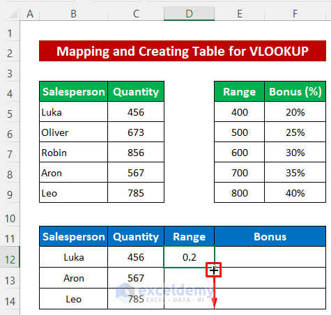
• Use the Fill handle tool to copy the formula to the cells below.

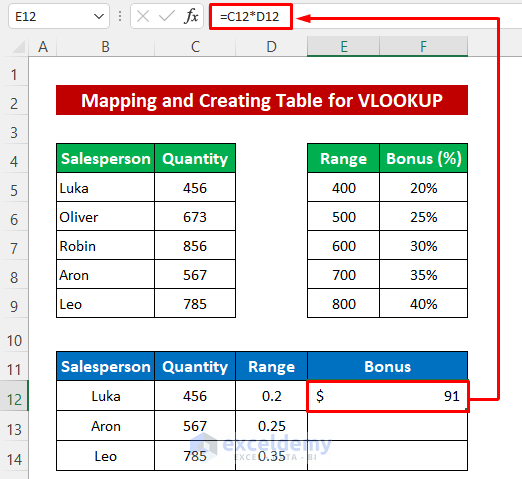
Finally, we’ll find the bonus amount.

• Enter the following formula in cell E12:

• Press Enter to return the output.

• Use the Fill Handle tool to fill the cells below.

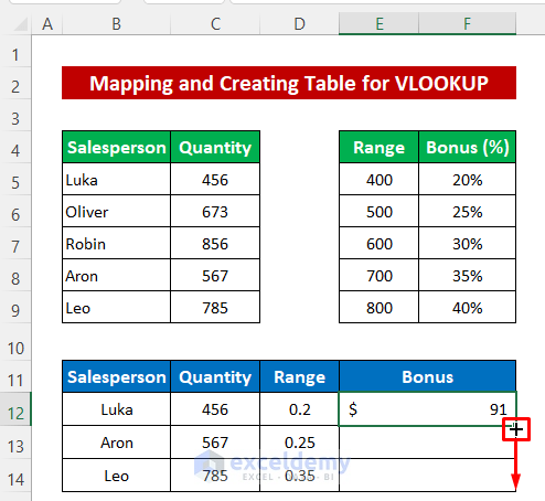
The bonus amount is evaluated using two table arrays.

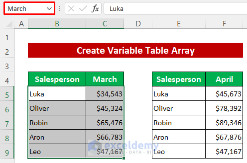
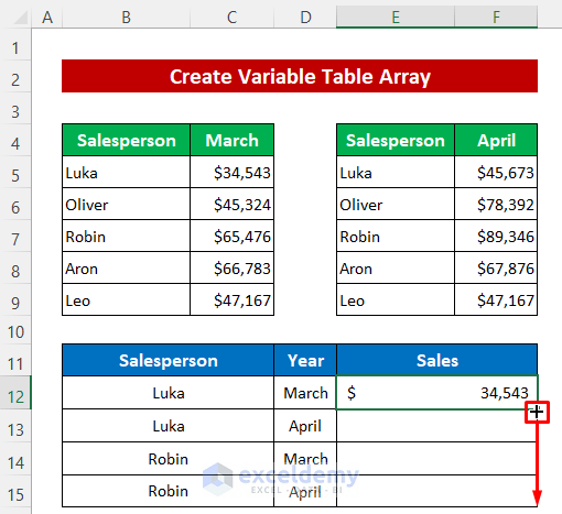
Example 3 – Creating a Variable Table Array

Lastly, we’ll create a variable table array for the VLOOKUP and INDIRECT functions. For this purpose, we modified the dataset again and made two tables to show the sales for two months. First, we’ll set named ranges for the tables.

Steps:

• Name the data range of the first table March.

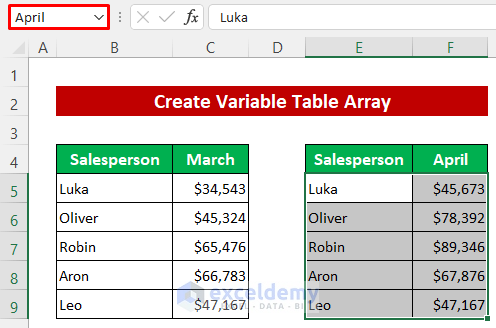
• Name the second table April.

Now let’s use these table arrays to get the sales of a salesperson from the two table arrays.

• Enter the following formula in cell E12:

• Press Enter.

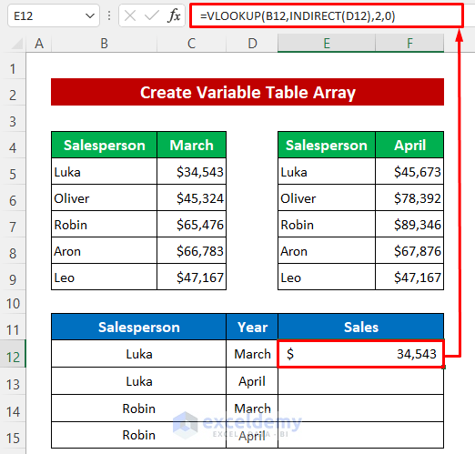
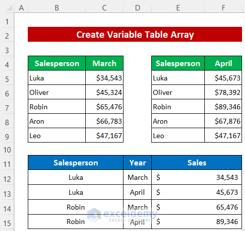
• Drag down the Fill Handle icon to copy the formula to the cells below.

The output is as in the image below.

Read More: Excel Table vs. Range: What Is the Difference?

Pros & Cons of Using Table Array in VLOOKUP

• Map with a single table if the data is from individual tables that are linked and related.
• If the tables are not connected, then there is no need to use a table array in VLOOKUP.
• Before using the formula, providing names for the table can simplify and reduce the syntax.
• More table arrays can be used for the VLOOKUP function.

Things to Remember

• It is useful to use VLOOKUP Table Array if the tables are co-related to each other.
• The Table Array must consist of 2 or more tables.

Download Practice Workbook

Related Articles

• How to Convert Range to Table in Excel
• Navigating Excel Table
• How to Make Excel Tables Look Good
• How to Convert Table to List in Excel
• Table Name in Excel: All You Need to Know
• How to Provide Table Reference in Another Sheet in Excel
• How to Insert Floating Table in Excel
• How to Make a Comparison Table in Excel

<< Go Back to Excel Table | Learn Excel