Types of Excel Tables: 3 Different Types

Method 1 – General Excel Table: Creation, Features, and Benefits

A. How to Create and Turn Off an Excel Table

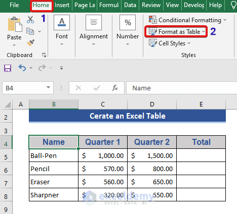
Step 1:

• Click on any cell in the dataset.
• Go to the Home tab.
• Select the Format as Table from the Styles tool.

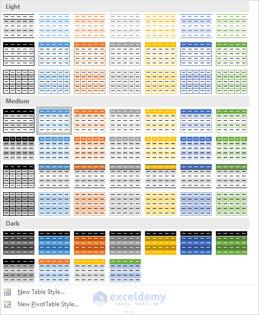
Step 2:

• Select any default table style.

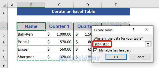
Or apply a keyboard shortcut Ctrl+T.

A new dialog box named Create Table will appear.

Step 3:

• Select the My table has headers if the data set has any headers.
• Press OK.

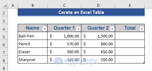
The following is our dataset after being converted to table format.

Turn off an Excel Table:

Step 1:

• From the Table Design tab, select the Convert to Range option.

A new pop-up will appear.

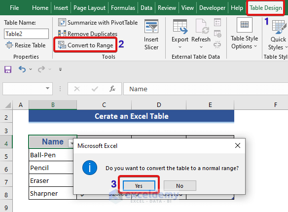
Step 2:

• Press Yes on the pop-up tab.

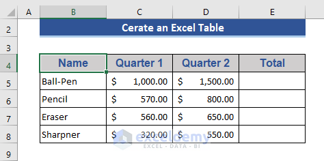
Our data is back to the primary state again. No more in a table format presented as a range.

B. Special Features/Operations of an Excel Table

1. Table Name

We can set the name of the table from the Table Name box. The name will be assigned by default.

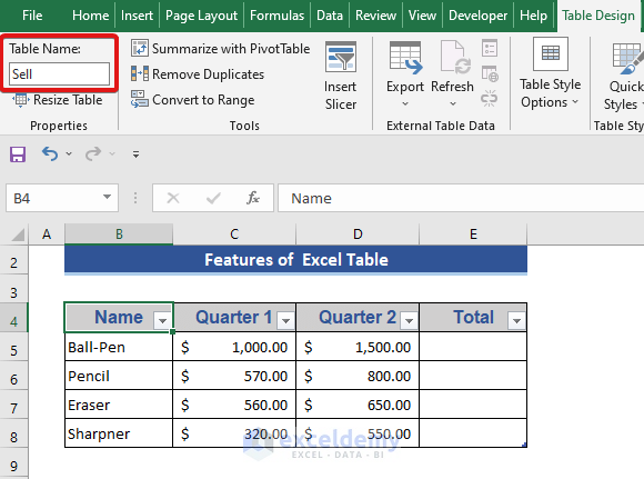
We can also rename a table name using the same option.

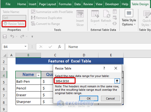
2. Resize Table Option

It has the Resize Table option, with which we can change the table size from the Properties option.

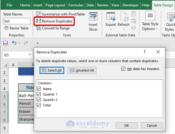
3. Remove Duplicates

Remove a Duplicate is an inbuilt option in the table that removes duplicates based on columns. We can also customize the selection of columns.

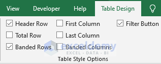
4. Table Styles Options

From the Table Styles Options, we can customize different options in the tab. A total of 7 options are here.

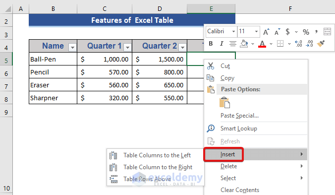
5. Insert Row and Columns and Expand Automatically

• Press the right button of the mouse.
• Choose the Insert option in the menu.
• From the option, select the desired location of a new row or column.

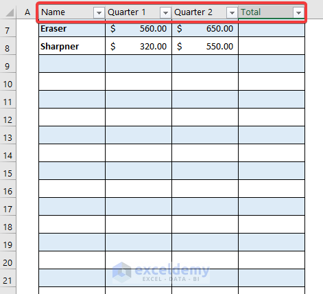
6. Header Visibility

Whenever you scroll down an Excel Table, the Table headers remain frozen. You don’t have to go to the top of the table each time to remember the header names.

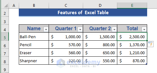
7. Easy Application of Formula

The formula is easily applied to the Excel table. Assume we want to get the total in cell E5.

• Just type the following formula in cell E5.

• Press Enter.

The next totals are automatically calculated, as shown in the figure below.

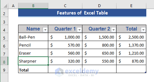
8. Subtotal Option

We can find the subtotal of the cells in column E by pressing Ctrl+Shift+T. This will add a row at the end and produce a subtotal value.

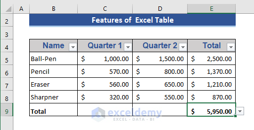
At cell E9, we will see a drop-down menu. This menu offers operations like average, maximum, minimum, etc.

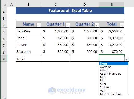
Select the SUM function for our use.

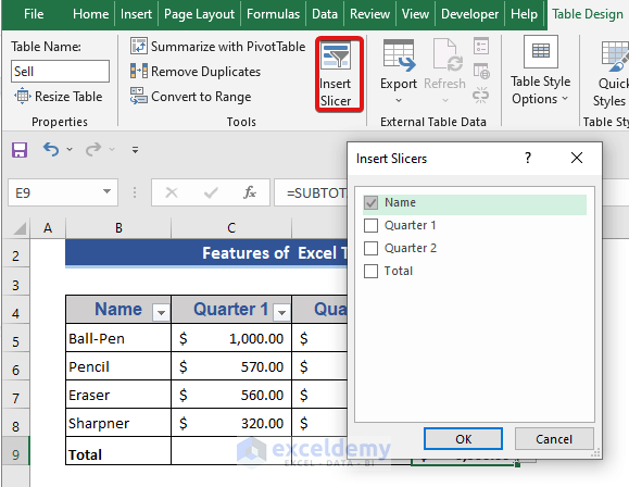
9. Insert Slicer

We also have the Insert Slicer option, which we get from the Table Design tab. Select Name from the slicer and press OK.

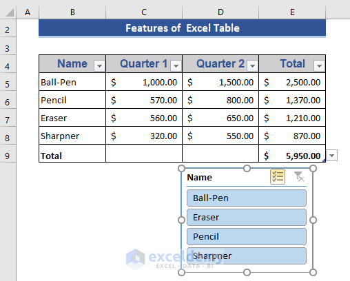
From the slicer, select any of the names.

• We chose Ball-pen in the slicer, and now data only shows for this item.

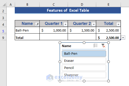
Slicer provides a shortcut to get the details of the specific item only.

C. Pros and Cons of an Excel table

Pros:

1. Header of the table, we can quickly sort and filter data.
2. The table can easily adjust rows and columns’ expansion or shrink.
3. Built-in subtotal functions reduce the use of formulas.
4. Formula fills up the adjacent cell, so you must use the formula for all cells.

Cons:

1. When any sheet is in a protected mood, table expansion will not work.
2. If any sheet contains a table, that sheet cannot be grouped with other sheets.
3. When using an Excel table, the custom view is not allowed.

Method 2 – Excel Pivot Table: Creation and Uses

A. How to Create a Pivot Table

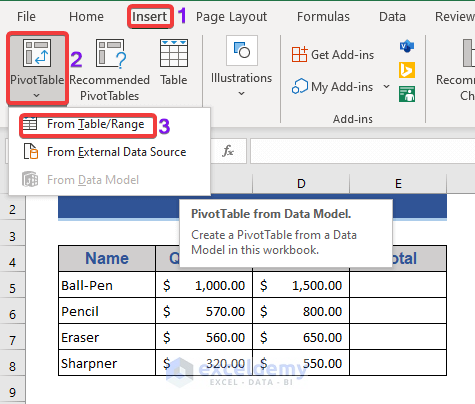
Step 1:

• Go to the Insert tab.
• Select PivotTable.
• Choose From Table/Range from the drop-down.

Step 2:

• Input the Table Range and Location.

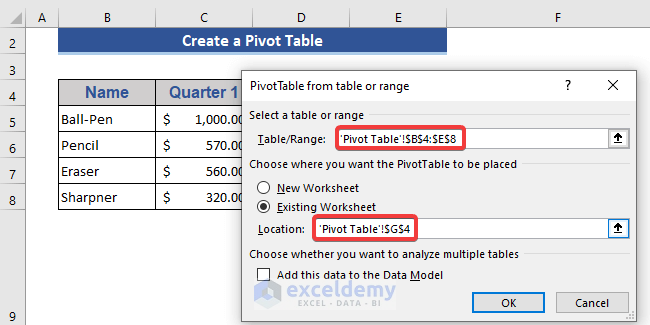
Step 3:

• Press OK.

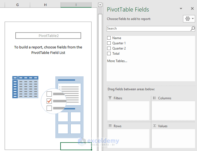
Step 4:

• Select objects from the PivotTable Fields.

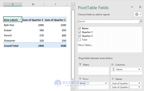
We can see a Grand Total row is added. We can customize the different fields of the Pivot Table.

B. Benefits of a Pivot Table

• Customize the Pivot table easily. Complex formulas are not needed here. Lots of options are available in the Pivot table field.
• Calculate in a short time using the Pivot table, as we do not need to apply any complex formula.
• Change the representation of data in a short time in the Pivot table. Even if we can make separate views using the same Pivot table.
• The pivot table is popular for its calculation accuracy. Due to the built-in functions, calculation accuracy is high.

C. An Example with the Excel Pivot Table

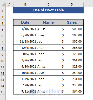
We will show the use of the Pivot table with detailed examples.  A new data set will be used to show the use of the Pivot table.

Step 1:

• Convert this data set into a Pivot table as the process is shown already.

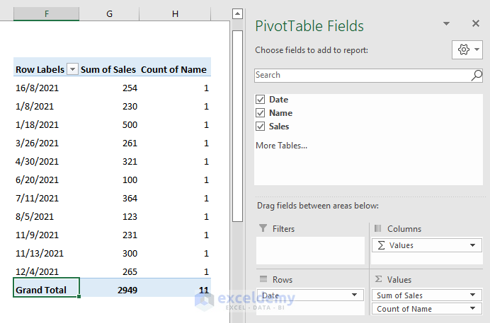
Change the calculation and representation by changing the PivotTable Fields.

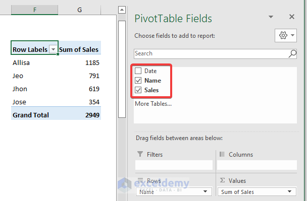
Step 2:

• Uncheck the Name option.

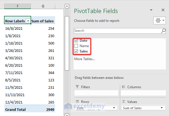
In this segment, we will represent the total sales of each customer.

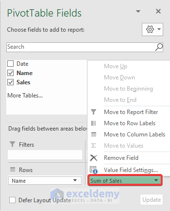
Step 3:

• Click on Sum of Sales.
• Select Value Field Settings.

Step 4:

• Select the Show Value As tab.
• Select % of Grand Total.

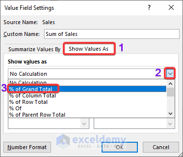
Step 5:

• Click OK.

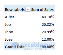
Now, see that tTWe have lots of options like the mentioned features in the Pivot table.

Method 3 – Excel Data Table: Creation and Uses

This is one of the most interesting types of Excel tables. There are two kinds of data tables available in Excel. In this section, we will discuss the creation of both data tables.

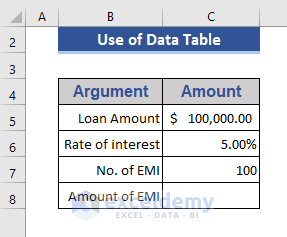
Calculate the Amount of EMI from different argument values. We applied the below formula for this purpose:

A. One-Variable Data Table

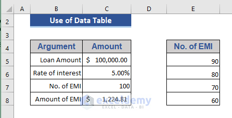
Step 1:

• Add a column with different values of EMI.

Step 2:

• The cell which contains the formula refers to that cell on cell E5.

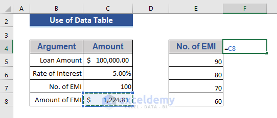
Step 3:

• Press the Enter button.
• Select the cells as shown in the image below.

Step 4:

• Go to the Data tab first.
• Select the Data Table from the What-If Analysis tab.

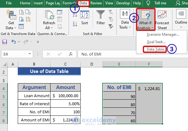
A new dialog box will appear.

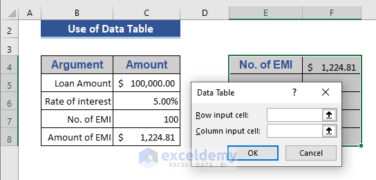
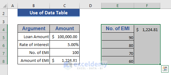
Step 5:

• In the Column input cell box, we will refer to the cell of the variable applied here.

Step 6:

• Press OK.

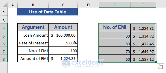
See that the EMI Amount for different No. of EMI is showing.

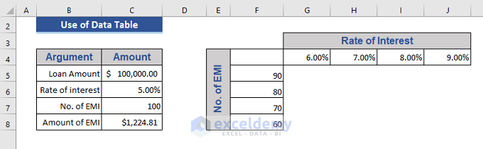
B. Two-Variable Data Table

Step 1:

• Use two variables here. Those are the Rate of Interest and EMI.

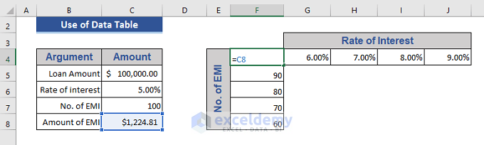
Step 2:

• Refer to the main formula on cell F5.

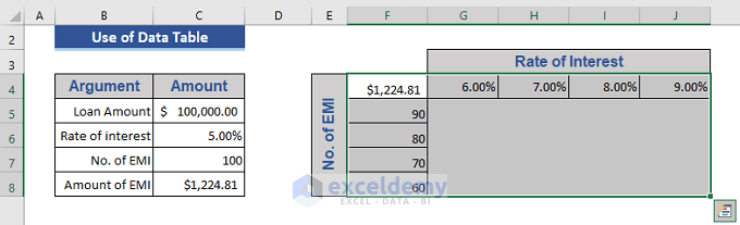
Step 3:

• Press Enter and select the cells where to apply the data table.

Step 4:

• Apply the data table tool from the previous method.
• A new dialog box appears.

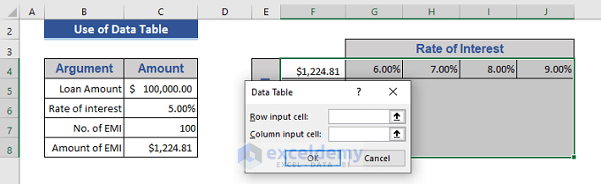
Step 5:

• Apply two cell references on the required field of the dialog box.

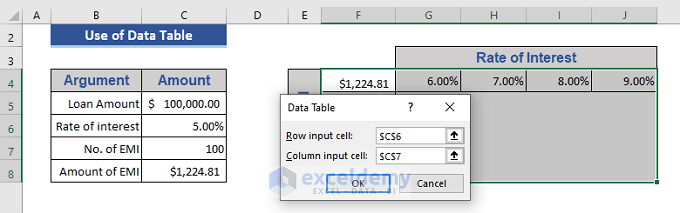
Step 6:

• Click OK.

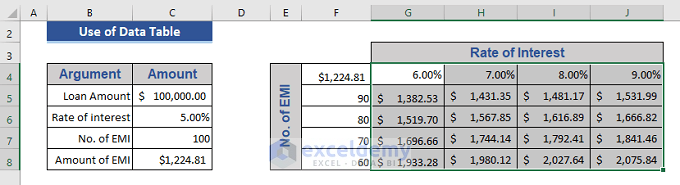
We applied two variables simultaneously using the data table.

Things to Remember

Some important things to keep in mind when we work with the table are:

1. No space is allowed in the Table name.
2. The table name is the combination of letters and numbers.
3. If any table name contains more than one word, it will be joined by an underscore.
4. The table name is always unique within the worksheet.
5. The maximum length of the table name is 255 characters.

Download Practice Workbook

Download this practice workbook to exercise while you are reading this article.

Further Readings

• Navigating Excel Table
• How to Convert Table to List in Excel
• How to Insert Floating Table in Excel
• How to Create a Table Array in Excel
• How to Provide Table Reference in Another Sheet in Excel

<< Go Back to Excel Table | Learn Excel