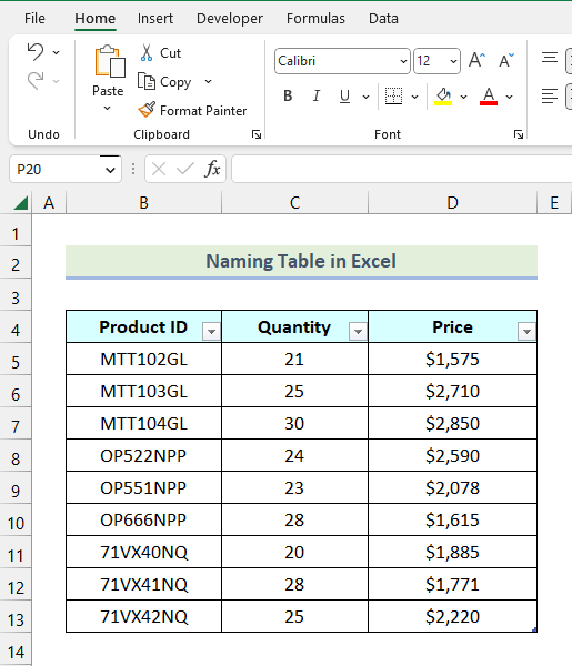
A table in Excel is a list of data with multiple rows and columns. What Excel tables offer more than a conventional data list is Excel tables facilitate more features such as sorting, filtering, etc. In this article, we are going to discuss five different ways to name a table in Excel. So, let’s start this article and explore these methods.
The following animated GIF demonstrates the overview of the methods that we will use in this article to name a table in Excel.
How to Create a Table in Excel?
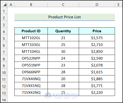
Creating an Excel table is quite easy and it’s just a matter of a few clicks. Excel enables us to transform a list of data into an Excel table. Now you are going to learn the process of creating an Excel table from a list of data. For demonstration, we will use the Product Price List as our dataset as shown in the image below.
To Create an Excel table from a list of data you need to follow the steps given below.
Steps:
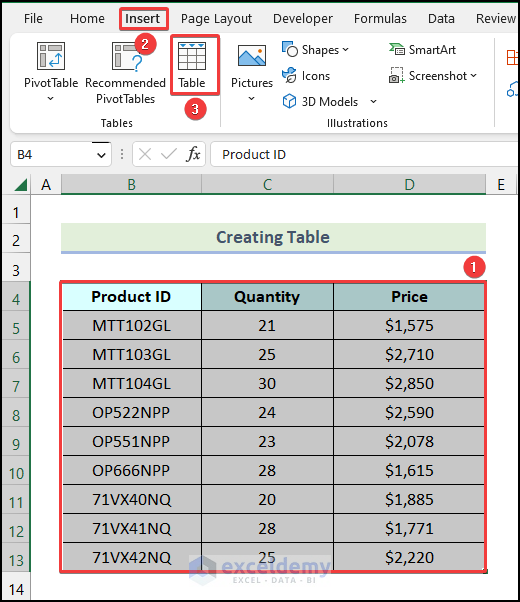
- Firstly, select the whole data list.
- Then, go to the Insert tab from the ribbon.
- After that click on the Table option.
Note: You can also use the keyboard shortcut CTRL + T to create a table.
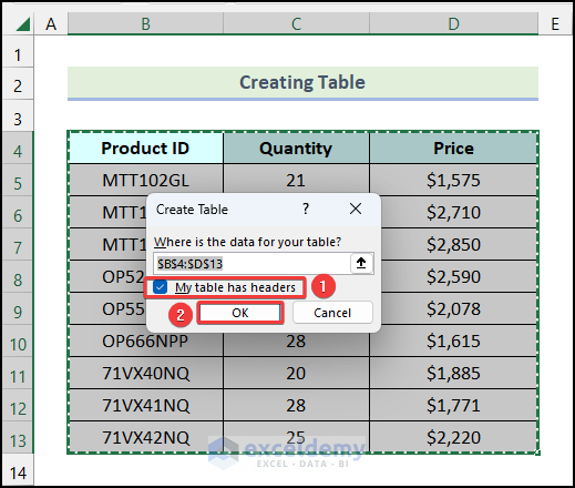
After following the process, a Create Table dialog box will appear on your worksheet.
- Now, make sure to check the field of My table has headers.
- Then, hit the OK command.
After hitting the OK command, you will see your data list has been converted into an Excel data table as in the picture below.
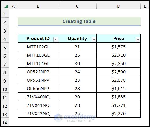
Table Naming Rules
There are the following restrictions that you need to consider while naming your Excel tables. Let’s get the rules one by one:
- You can’t use the same table name over and over again. That is, all of the table names have to be unique.
- Spaces between two consecutive words are not allowed while naming your Excel tables. You can use an underscore to link the words if necessary.
- You cannot use more than 255 characters in your table name. This means using too lengthy table names is strictly prohibited.
- At the start of each table name, you can use either a letter, an underscore, or a backslash(\).
- You cannot use a cell reference as your table name.
Name Table in Excel: 5 Simple Methods
In this section of the article, we will learn five easy methods to name a table in Excel. Not to mention, we used the Microsoft Excel 365 version for this article; however, you can use any version according to your preference.
So, without having any further discussion let’s dive straight into all the methods one by one.
1. Using Table Name Box to Name Table
If you want to rename your table immediately after creating them, only then you can use this option. Because the Table Design tab becomes visible just after creating a new table. Other times this tab becomes invisible. You need to select the entire table to make this tab visible again. So when you are done with creating a new table, follow the steps given below.
Steps:
- Firstly, select the entire table.
- After that, go to the Table Design from Ribbon.
- Now, click on the Table Name box in the Properties group as marked in the following image.
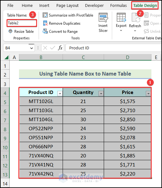
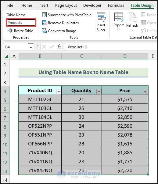
- Following that, edit your table name within the Table Name box. In this case, we renamed the table as Products.
Read More: Does TABLE Function Exist in Excel?
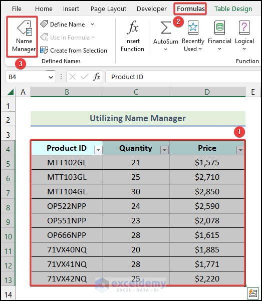
2. Utilizing Name Manager
There’s an alternative way that you can use to change your table name at any moment. It is by utilizing the Name Manager option. Now, let’s use the steps outlined below to do this.
Steps:
- Firstly, select the entire table and go to Formulas tab from the ribbon.
- After that, choose the Name Manager option from the Defined Names group.
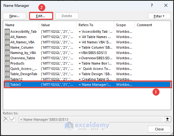
After hitting the Name Manager command, the Name Manager window will pop up. From the pop-up window.
- Now, select your table name.
- Then hit the Edit option.
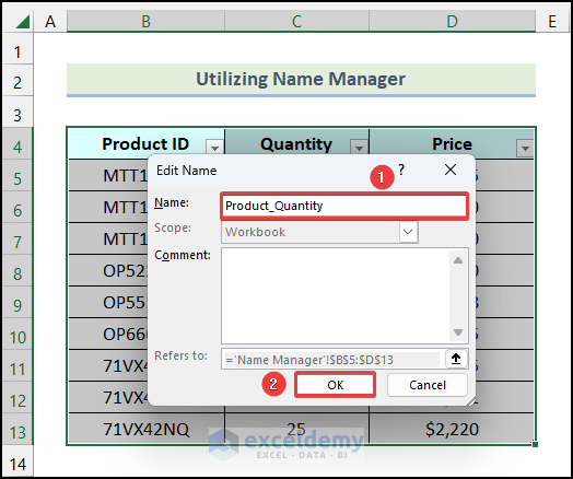
After that, another dialog box named Edit Name will appear. From the dialog box,
- Subsequently, insert the table name within the Name box.
- Finally, hit the OK command.
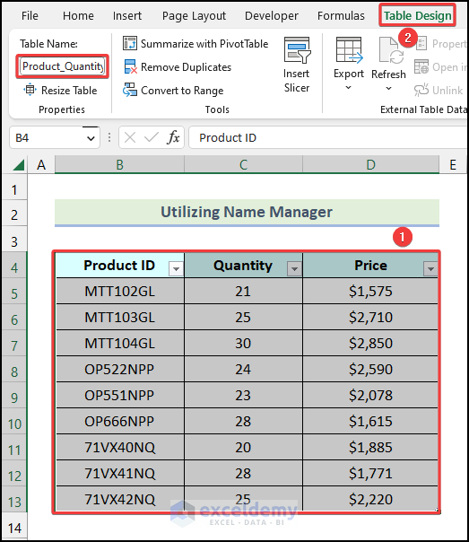
- Next, the Name Manager dialogue box will reappear on your worksheet, and click on the Close option.

- Now, select the table and go to the Table Design tab.
Consequently, you will see that the name of the table is changed as demonstrated in the following image.
Read More: Excel Table vs. Range: What Is the Difference?
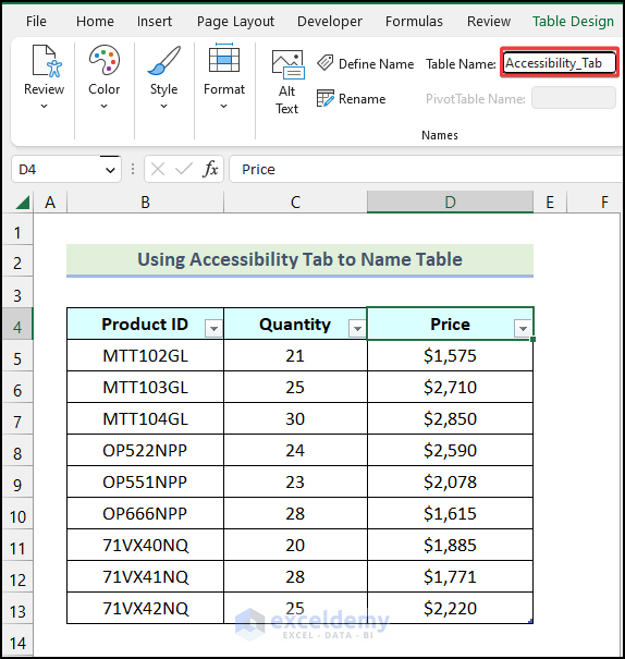
3. Using the Accessibility Tab to Name Table
Using the Accessibility tab is another smart way to name a table in Excel. Now, let’s follow the steps discussed in the following section to do this.
Steps:
- Firstly, select the entire table and go to the Review tab from ribbon.
- After that, click on the Check Accessibility option from the Accessibility group.

- Consequently, the Accessibility tab will open, and click on the Table Name field in the Names group.
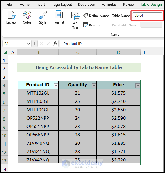
- Now edit the name of the table and your table name will be changed. Here, we used Accessibility_Tab as the table name.
Read More: How to Convert Range to Table in Excel
4. Utilizing the Quick Access Toolbar
We can also name a table in Excel by using the Quick Access Toolbar option. To do this, you need to follow the instructions outlined below.
Steps:
- Firstly, select the entire table and go to the Table Design tab from the ribbon.
- Following that, right-click on the Table Name field as shown in the image below.
- Then, choose the Add to Quick Access Toolbar option.
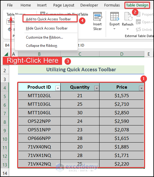
Consequently, the Table Name field will be added to the Quick Access Toolbar.

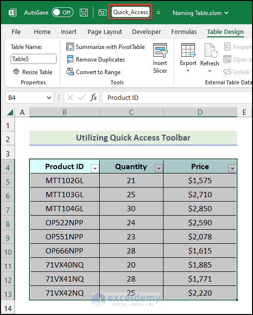
- Subsequently, click on the newly created Quick Access Toolbar and change the name of the table.
Read More: Navigating Excel Table
5. Incorporating VBA into Name Table
Incorporating VBA is another efficient way to name a table in Excel. For demonstration initially, we have set the name of the table as Table_Name. Now, we will change this table name using the VBA Macro feature. So, let’s use the process discussed in the following section.
- Firstly, go to the Developer tab from Ribbon. It is not displayed in the ribbon by default. You have to enable the Developer tab from Excel Options.
- Then, choose the Visual Basic option from the Code group.
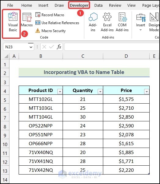
As a result, the Microsoft Visual Basic for Applications window will open on your worksheet.

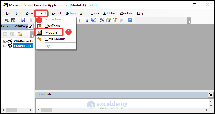
- Subsequently, go to the Insert tab in the Microsoft Visual Basic for Applications window.
- Then, choose the Module option from the drop-down.
Step 02: Write and Save VBA Code
- After that, write the following code in the newly created Module.
Sub Name_Table_VBA()
Dim old_name As String, new_name As String
old_name = "Table_Name"
new_name = "Naming_by_VBA"
With ActiveSheet
.ListObjects(old_name).Name = new_name
End With
End Sub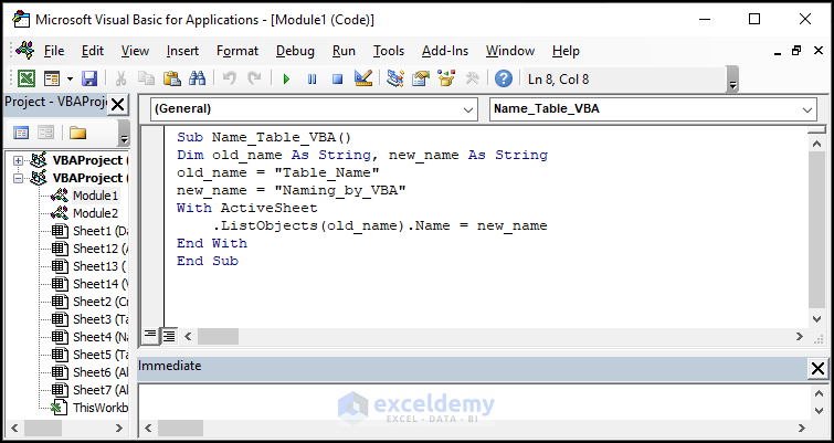
Code Breakdown
- Firstly, we created a sub-procedure named Name_Table_VBA.
- After that, we introduced two variables named old_name, and new_name as String.
- Subsequently, we assigned the “Table_Name” to the old_name variable.
- Then, we assigned the “Naming_by_VBA” to the new_name variable.
- Now, we used a With statement to change to name of the table of the active worksheet.
- Subsequently, we ended the With statement.
- Finally, we ended the sub-procedure.
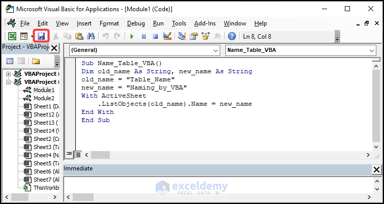
- Then, click on the Save option.
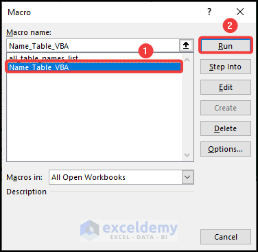
Step 03: Run Created Macro
- Firstly, use the keyboard shortcut ALT + F11 to return to the worksheet.
- Then, select the entire table and apply the keyboard shortcut ALT + F8 to open the Macro dialogue box.
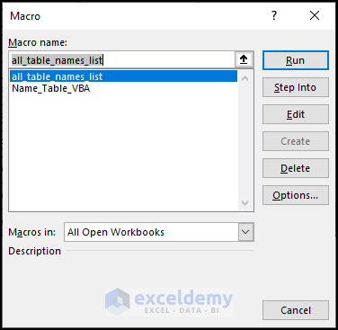
- Now, choose the Name_Table_VBA option.
- Finally, click on Run.
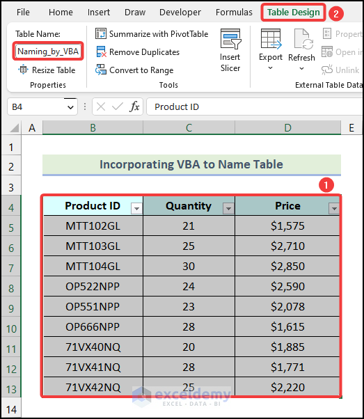
- Now, select the entire table and go to the Table Design tab.
You will see that the name of the table is changed as demonstrated in the following picture.
Read More: How to Make Excel Tables Look Good
How to Rename a Table Column in Excel
To change your table column name, you don’t need to go through a load of hassles. All you need to do is explained in the following section.
Steps:
- Firstly, select a table column header where you want to bring changes. In this case, we have selected the Price Column.
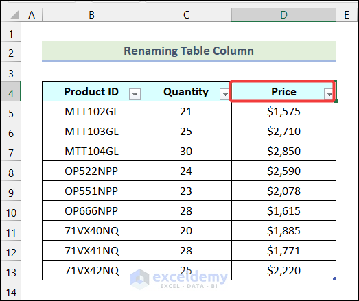
- Now, double-click on the existing name and wipe out the already existing name on it.
- Following that, type your new column name. Here, we used Current Price as the new column header.
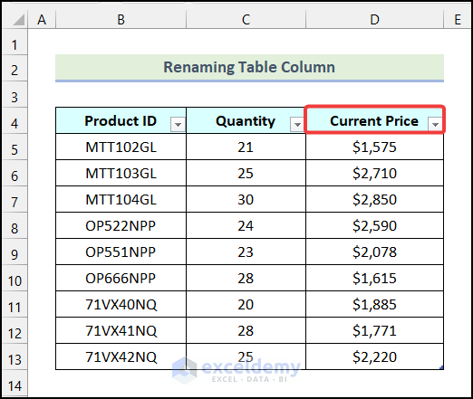
That’s simply what can be done. Bingo!
Read More: How to Convert Table to List in Excel
How to Get a List of All Table Names in Excel
There are multiple ways that you can use to get a list of all the table names in Excel. So, let’s discuss them all one by one.
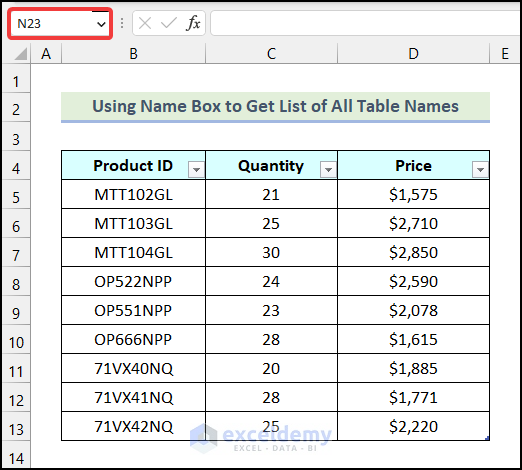
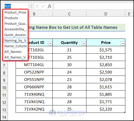
1. Using Name Box to Get List of All Table Names
This is the quickest way to display all the table names throughout your Excel workbook. You can easily find the Name Box on the left side of the formula bar. Now, let’s use the steps mentioned below to do this.
Steps:
- Firstly, click on the Name Box option at the top-left corner as shown in the image below.
- Consequently, You will see a drop-down arrow within the Name Box. Just click on the drop-down arrow.
That’s all you need to get a list of all the table names throughout your Excel workbook.
Read More: Types of Tables in Excel: A Complete Overview
2. Implementing VBA Code to Get List of All Table Names
You can also use the VBA code to get a list of all the table names. So, let’s follow the instructions given below to do this.
Steps:
- Firstly, use the steps mentioned in Step 01 of the fifth method to create a new Module.
- Following that, write the following code in the newly created Module.
Sub all_table_names_list()
Dim a As ListObject
Dim b As Worksheet
Dim c As Long
c = -1
For Each b In Worksheets
For Each a In b.ListObjects
c = c + 1
Sheets("All Names VBA").Range("B16").Offset(c).Value = a.Name
Next a
Next
End Sub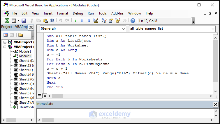
Code Breakdown
- Firstly, we created a sub-procedure named all_table_names_list.
- Then, we introduced three new variables.
- Next, we set the value of the variable c to -1.
- After that, we used two nested For Next loops to find all the names of the tables.
- Following that, we closed the For Next loops.
- Finally, we ended the sub-procedure.
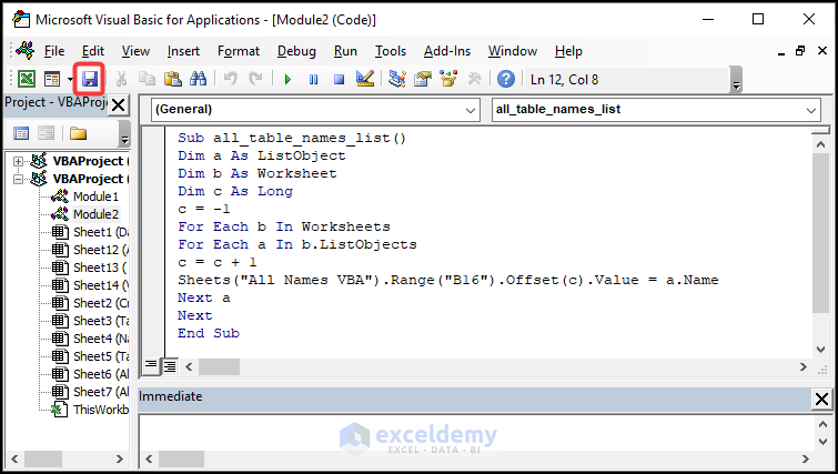
- After writing the code, click on the Save option
- Now, apply the keyboard shortcut ALT + F11 to return to the worksheet.
- Afterward, choose the entire table and use the keyboard shortcut ALT + F8 to open the Macro dialogue box.
- Following that, choose the all_table_names_list option.
- Lastly, click on Run.

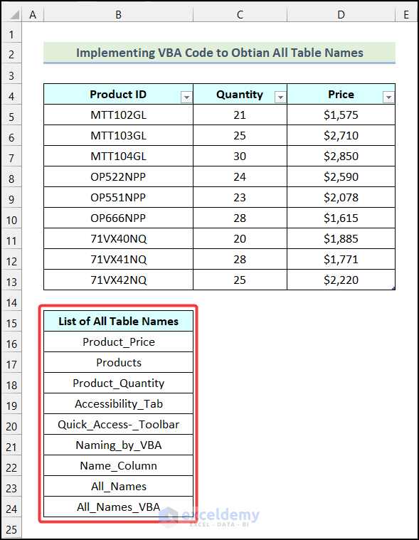
Consequently, the list of all table names will be shown on your worksheet as shown in the picture below.
Download Practice Workbook
You are recommended to download the Excel file and practice along with it.
Conclusion
To sum up, we have discussed all the facts that you need to know about table names in Excel. You are recommended to download the practice workbook attached along with this article and practice all the methods with that. And don’t hesitate to ask any questions in the comment section below. We will try to respond to all the relevant queries ASAP.
Further Readings
- How to Insert Floating Table in Excel
- How to Make a Comparison Table in Excel
- How to Create a Table Array in Excel
- How to Provide Table Reference in Another Sheet in Excel
<< Go Back to Excel Table | Learn Excel
Get FREE Advanced Excel Exercises with Solutions!
