In Microsoft Excel, a Table is a tremendously instrumental tool to process large amounts of data with ease. It saves a lot of time and reduces a lot of stress while analyzing data. Though there is no such built-in Excel function named TABLE in truth, we can create an Excel table using VBA macros. Besides, we can also make an Excel table using the built-in Table command. There is also another table, the Data table, used for What-if analysis. Our article will cover all these with suitable examples and illustrations.
Creating a Table with VBA and Excel Command
We can create an Excel table using both VBA Macros and an Excel command.
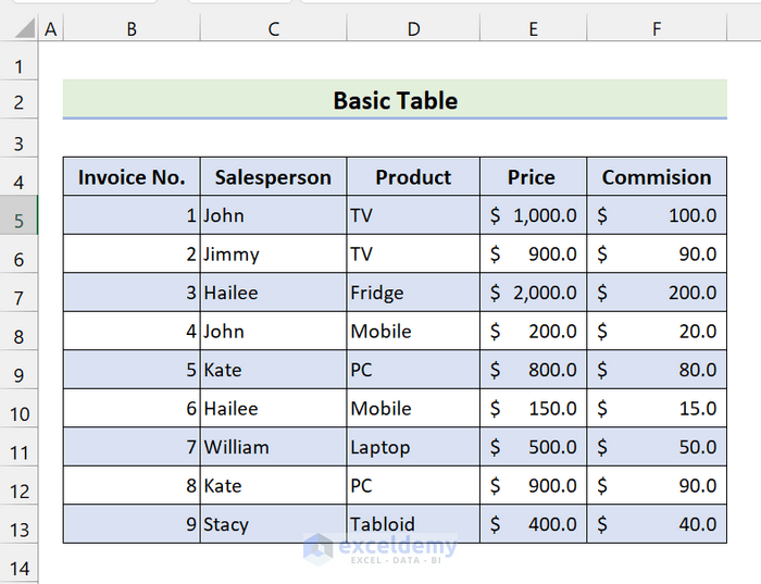
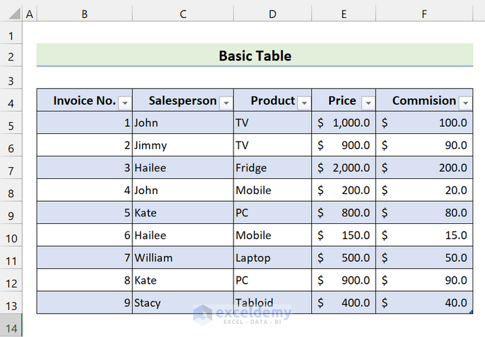
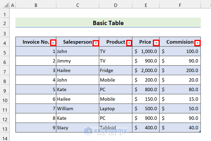
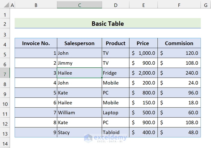
Look at the following dataset. We will use this all through our tutorial as the sample dataset.
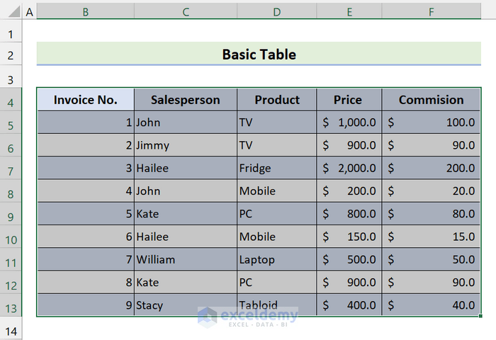
Now, if you convert this into a table, it will look like this:
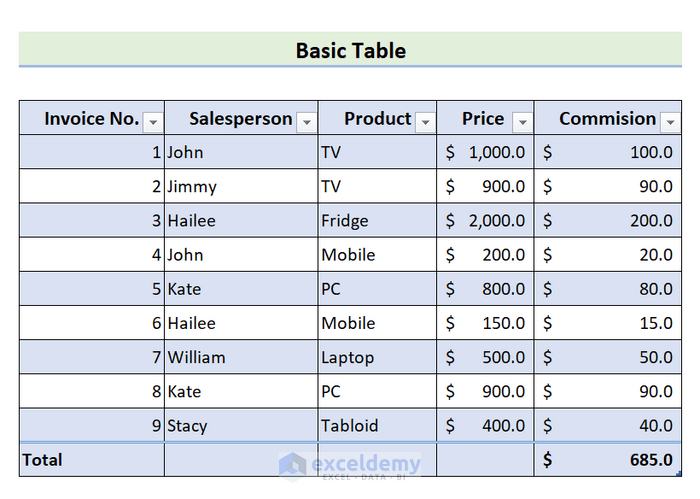
This is an Excel Table. It has a lot of functionality, which we will discuss later. Before that, let’s see first how to form an Excel table using VBA or built-in Excel commands.
So, there are two ways to make an Excel table: manually using an Excel command or using the VBA codes and creating a suitable function.
1. Create a Function for an Excel Table Using VBA Codes
Here is how we can create a function using VBA macros and create an Excel Table.
📌 Steps
1. First, press ALT+F11 on your keyboard to open the VBA editor.
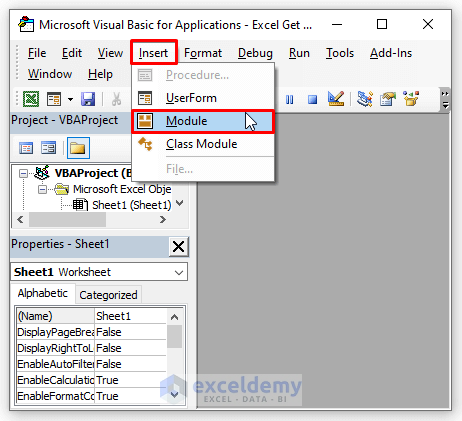
2. Click on Insert > Module.
3. Then, type the following code:
Sub CreateTable()
Sheet1.ListObjects.Add(xlSrcRange,Range("B4:F13"), ,xlYes).Name ="Table1"
End Sub
4. Save the file.
5. Then, press ALT+F8. It will open the Macro dialog box.
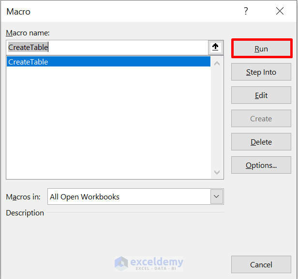
6. Click on Run.
Finally, we are successful in creating a table using VBA codes.
Read more: Types of Tables in Excel
2. Create an Excel Table Using Built-in Excel Command
Here, you can create a table using a keyboard shortcut or using the Table command from the Insert tab.
Using Keyboard Shortcut:
📌 Steps
1. First, select the range of cells B4:F13
2. Then, press Ctrl+T on your keyboard. You will see a Create Table dialog box.
3. In the box, your range of cells is already given. Now, select My table has headers box option.
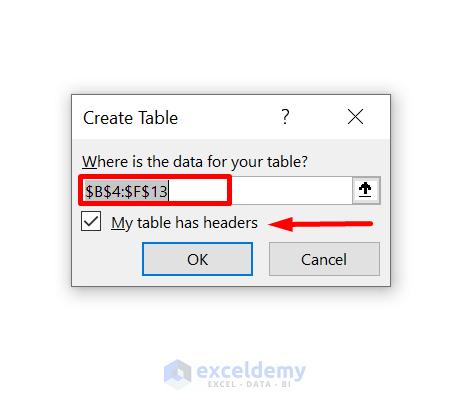
4. Click on OK.
As you can see, we have converted our dataset into a table.
Using The Table Command from the Insert Tab:
📌 Steps
1. First, select the range of cells B4:F13
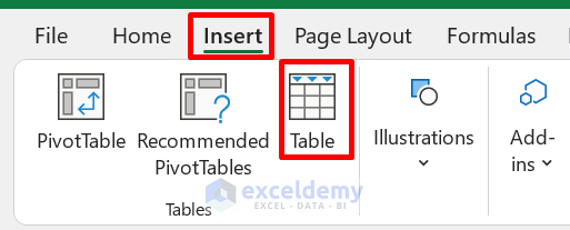
2. Now, go to Insert Tab. Click on Table. You will see a Create Table dialog box.
3. In the box, your range of cells is already given. Now, select My table has headers box option.
4. Click on OK.
Read more: How to Create a Table Array in Excel
The Functionality of an Excel Table
An Excel table is multidimensionally useful. In the following discussion, we will discuss some of its basic applications. Let us see one by one.
1. Sort
We know what sort is in Excel. Previously we had to do sorting manually with the help of the Data tab. Now, on our table, the sorting is enabled automatically. You can see the dropdown menu after each column.
Now, we are going to sort the table based on the Price (largest to smallest).
📌 Steps
1. Click on the dropdown of the column Price.
2. Select Sort Largest to Smallest option.
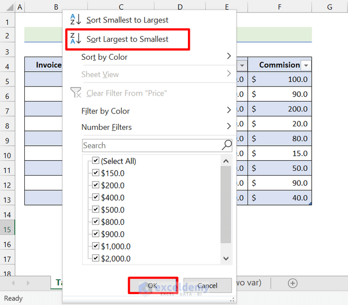
3. Click on OK.
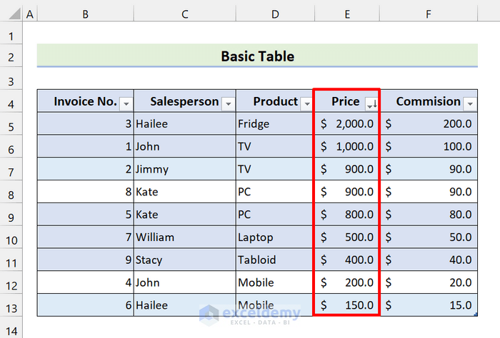
Here, we sorted our table based on Price.
2. Filter
You can also filter data based on any values. Here, we are filtering the table based on the salesperson John.
📌 Steps
1. Select the dropdown of the Salesperson column.
2. In the Filter option, first, uncheck the box Select all. Then, check the box of John.
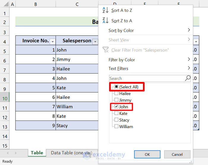
3. Click on OK.
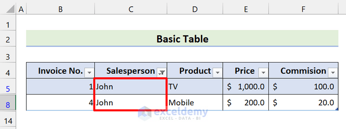
Now, we have filtered our table based on the salesperson John.
Read More: Excel Table vs. Range: What Is the Difference?
3. AutoFill Formulas
In a dataset, we use formulas to perform any calculation. Then we have to drag that formula across all the columns or rows to copy that. But, at the table, you don’t have to do all these kinds of stuff. All you have to do is insert the formula. And our table will auto-fill the column.
In our previous table, the Commission column was calculated based on 10% of the product price. Here, we are changing it to 15%. After that, the Commission column will be auto-filled.
📌 Steps
1. Type the following formula in Cell F5:
=(E5*15)/100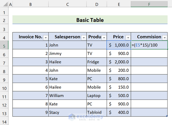
2. Press Enter.
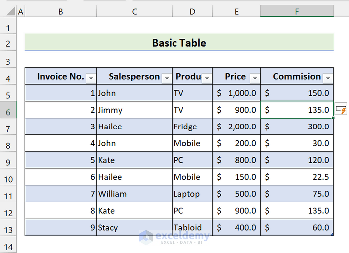
As you can see, the formula is automatically filled throughout the column.
Similarly, if you change the formula in any column, all the columns will be changed accordingly.
Read More: How to Convert Range to Table in Excel
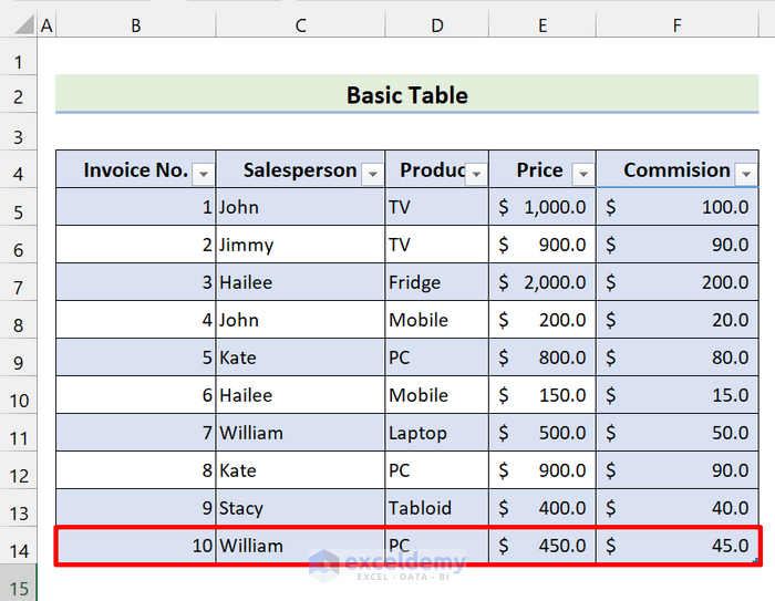
4. Expand Automatically for New Rows/Columns
When we add new rows or columns, the table automatically adds them as a table entry.
Read More: Navigating Excel Table
5. Perform Operations without Formulas
Every table has an additional option Total Row. You can perform SUM, COUNT, MIN, MAX, etc. operations without inserting any formulas. To enable this, press Ctrl+Shift+T on your keyboard. After that, a new row called Total will be added.
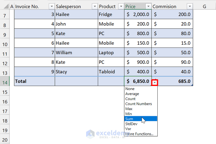
Here, we find the total sum of the column Price.
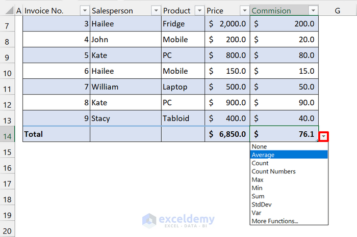
Again, the average of the Commission will be:
Read More: How to Make Excel Tables Look Good
6. Easy Legible Formulas
In a table, formulas are human-readable. Anyone can interpret these formulas. Take a look at this image:
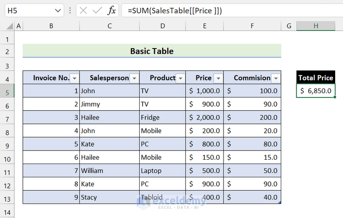
Here, the formula describes the total SUM of the column Price in SalesTable.
Read More: How to Convert Table to List in Excel
7. Structured References with Manual Typing
Suppose you want to find the min value of the Commission. You don’t have to select the whole column ranges in the formula. All you have to do is select the table name and the column name.
Here, our table name is SalesTable.
Type the following formula in any cell:
=Min(SalesTable[Commision])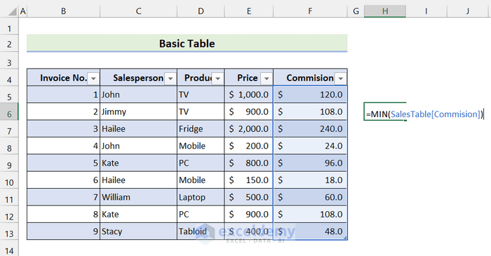
As you can see, our range is automatically selected.
Change Excel Table Properties
There are many properties of a table. We are only discussing the basic properties of a table and how you can change them.
1. Change Formatting of a Table
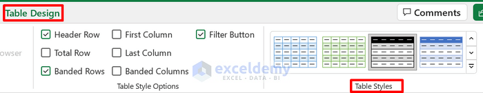
You can change your table formatting in the Table Design tab. Just click any cell of your table. Then, go to the Table Design tab. In the Table Style option, you will see various table formats.
Click on the down arrow to expand all the Table Styles.
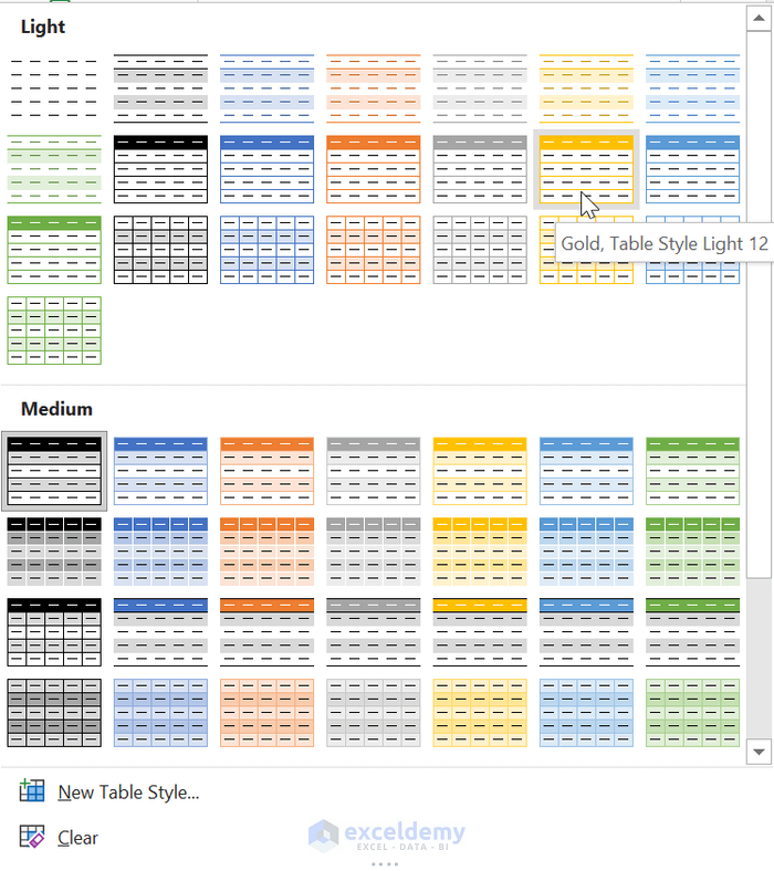
You can choose any of them to format your table.
2. Remove Formatting of a Table
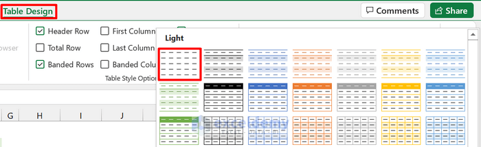
Now, you may want to change the format and go back to the basic format which you created. Go to the Table Design > Table Styles.
After that, choose None
3. Select Default Table Style
You can also select a default table style. You can use this style whenever you create a table. Just Right-click any of the cell styles and select Set As Default.
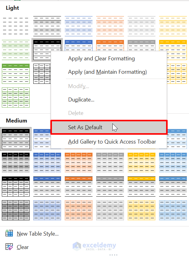
Now, a new table of this same workbook will have this style.
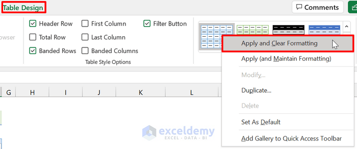
4. Clear Local Formatting
When you implement a table style, local formatting is saved by default. However, you can optionally cancel local formatting if you require. Right-click any style and choose “Apply and Clear formatting“:
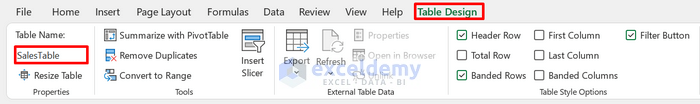
5. Rename a Table
When you create a table, the name of the table will be set automatically. It will look like Table1, Table2, etc. To rename a table in Excel, go to the Table Design tab. Then, you will see the Table Name box. Here, you can change and give your table any name.
Read More: Table Name in Excel: All You Need to Know
6. Get Rid of a Table
To change the table into the normal dataset, go to the Table Design tab > tools. Click on Convert to Range. Then, click on Yes.
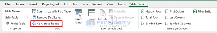
After that, it will convert our table into the normal dataset.
The Data Table in Microsoft Excel
A data table is a range of cells in which you can modify values in some of the cells and come up with different answers to a problem. This is one of the What-If Analysis tools that enables you to try out distinct input values for formulas and see how changes in those values affect the output of the formula.
1. Create Data Table Function with One Variable in Excel
A data table with one variable lets us test a range of values for a single input. We test the range of values with the change of that input. If there is any change in the input, it will change the output accordingly.
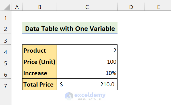
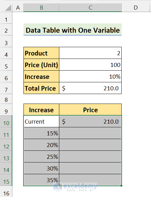
Here, we have some data about a product. There are 2 products, and the per unit price is $100. If the price increases by 10%, the total price will be $210.
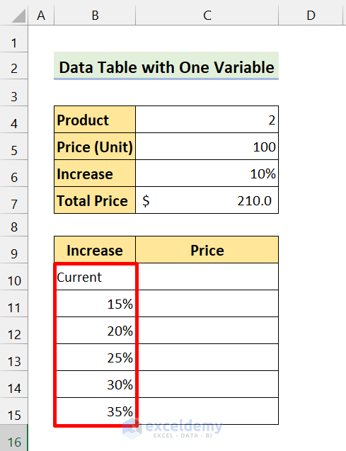
Now, we will create a data table with the variable increase. We will analyze increasing the total price after the percentages rise to 15%, 20%, 25%, 30%, 35%.
📌 Steps
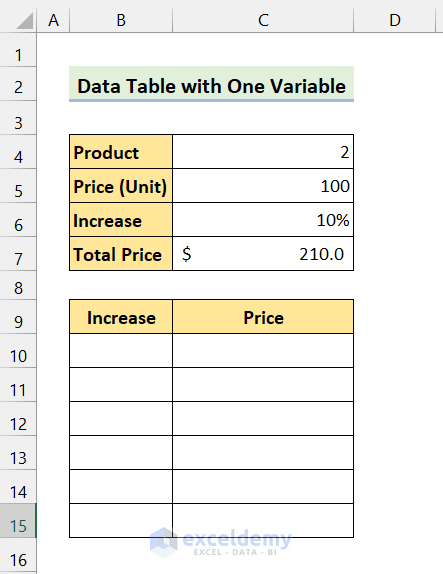
1. First, create two new columns, Increase and Price.
2. Then type the following in the Increase Column.
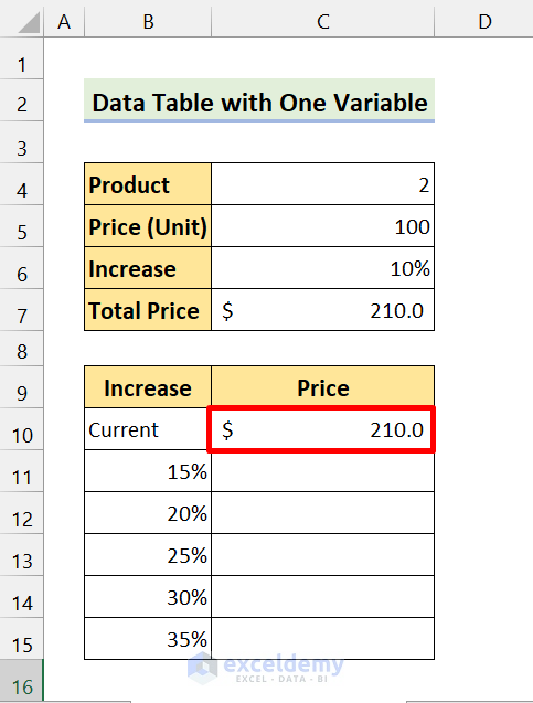
3. In cell C10, type =C7. Then press Enter. You will see the current Total price.
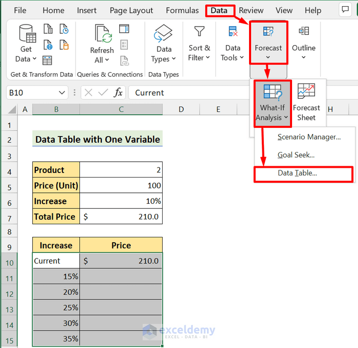
4. Now, select the range of cells B10:C15
5. Go to the Data Tab. Then you will find the Forecast option. Click on What-If Analysis > Data Table.
6. After that, the Data Table dialog box will appear. In the Column input cell box, select the Increase percentage.
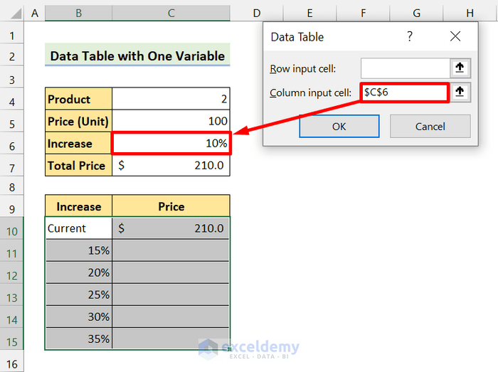
7. Click on OK.
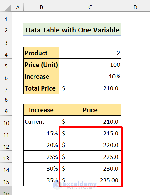
Finally, you can see all the possible total prices after increasing the percentages from the data table with one variable.
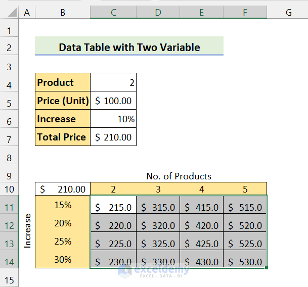
2. Create Data Table Function in Excel with Two Variable
The data table with two variables is almost similar to the previous one. Here, two variables affect the output. In other words, it explains how changing two inputs of the same formula changes the output.
We are using the same dataset as the previous one.
📌 Steps
1. First, create new rows and columns like the following:
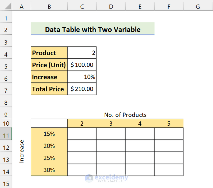
2. Now, in cell B10, type =C7.
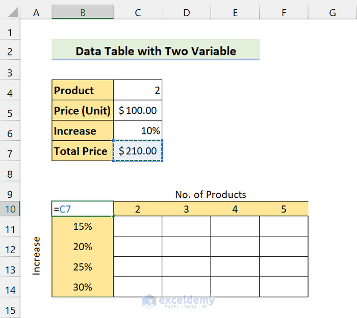
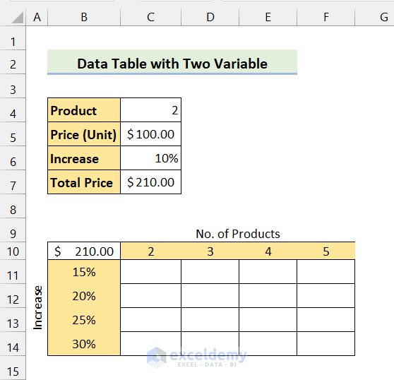
3. Press Enter. It will show the total price.
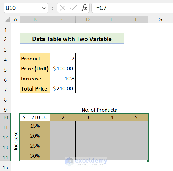
4. Next, select the range of cells B10:F14
5. Now, go to the Data tab. From the Forecast option, click on What-If Analysis > Data Table.
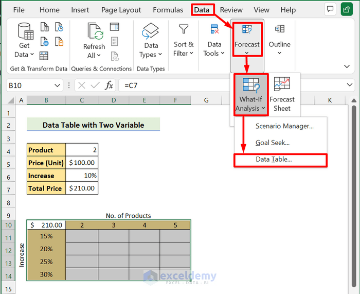
6. After that, a Data Table dialog box will appear. Select Number of products in the Row input cell box and Increase the percentage in the Column input cell shown below:
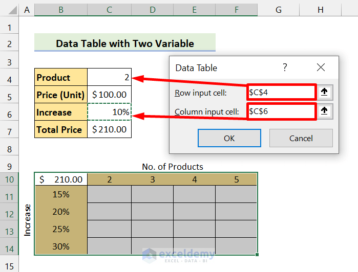
6. Then, click on OK.
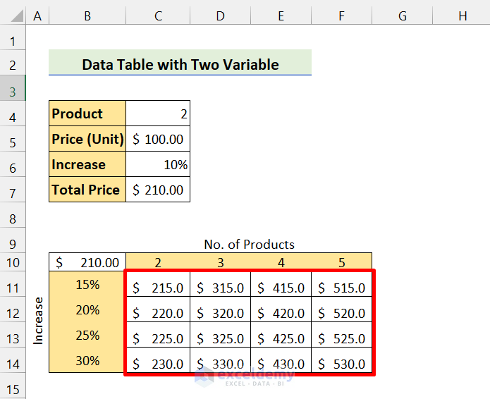
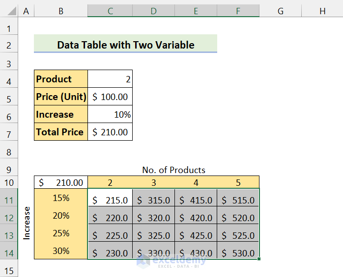
Finally, you will see all the possible prices for increasing the percentages as well as the number of products. Change in the Increase and No. of Products affect the total price.
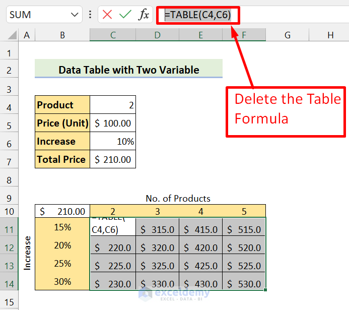
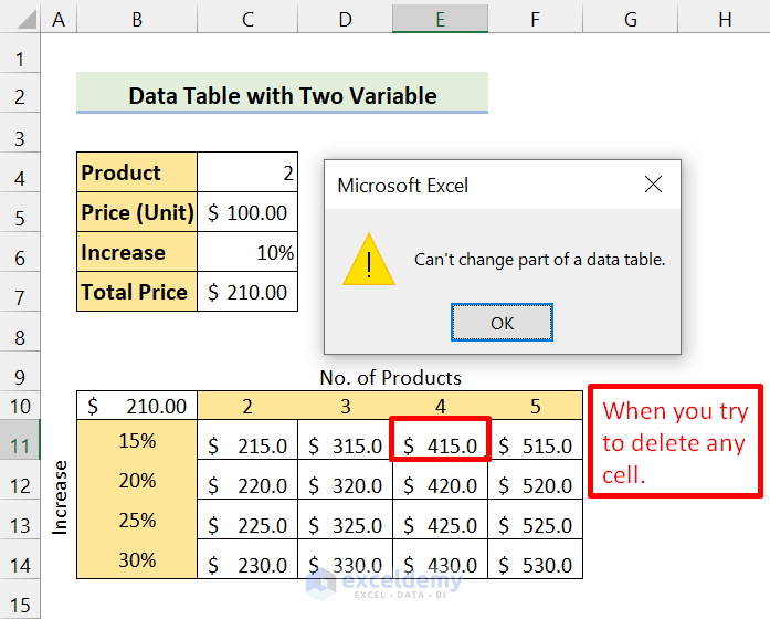
3. Edit Data Table Results in Excel
Now, you cannot change any part of the table of individual values. You have to replace those values by yourself. Once you start editing the data table, all those calculated values will be gone. After that, you have to edit each cell manually.
📌 Steps
1. First, select all the calculated cells. We are selecting the range of cells C11:F14.
2. Then, delete the TABLE formula from the formula bar.
3. After that, type a new value in the formula bar.
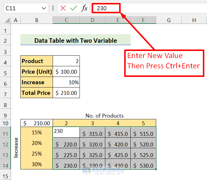
4. Then, press Ctrl+Enter.
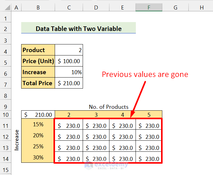
In the end, you will see your new value in all cells. Now, all you have to do is edit this manually. By this method, you have converted it to a normal range.
4. Recalculate Data Table Function in Excel
Now, your formulas will slow down your Excel if it contains a large data table with multiple variables. In such cases, you have to disable automatic recalculations in that and all other data tables.
First, go to the Formulas tab. From the Calculation group, click on Calculation Options > Automatic Except for Data Tables.
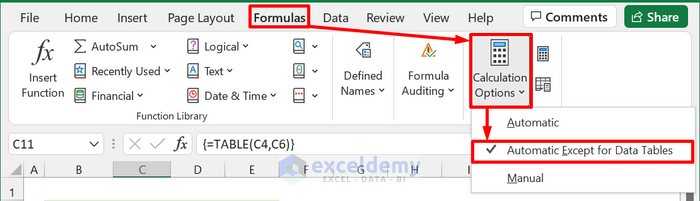
This method will turn off automatic data table calculations and make your recalculations of the entire workbook.
5. Delete a Data Table
Now, Excel does not allow the deletion of values in particular cells holding the results. An error message “Cannot change part of a data table” will show up if you try to do this.
However, you can simply delete the whole array of the calculated values.
📌 Steps
1. First, select all the calculated cells.
2. Then, press Delete on your keyboard.
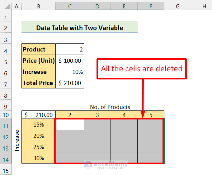
As you can see, it deleted all the resulting cells of the data table
💬 Things to Remember
✎ To create a data table, the input cell(s) must be on the same sheet as the data table.
✎ In the data table, you cannot change or edit a particular cell. You have to delete the whole array.
✎ In the normal table, if you change the formula in any column, the entire column will be changed accordingly.
Download Practice Workbook
Download this practice workbook.
Conclusion
To conclude, I hope this tutorial has provided you with a piece of useful knowledge about tables in Excel. We recommend you learn and apply all these instructions to your dataset. Download the practice workbook and try these yourself. Also, feel free to give feedback in the comment section. Your valuable feedback keeps us motivated to create tutorials like this.
Further Readings
- How to Insert Floating Table in Excel
- How to Make a Comparison Table in Excel
- How to Provide Table Reference in Another Sheet in Excel
<< Go Back to Excel Table | Learn Excel
Get FREE Advanced Excel Exercises with Solutions!
