How to Make Excel Tables Look Good (8 Effective Tips)

Written by Taryn Nefdt

Last updated: Jul 3, 2024

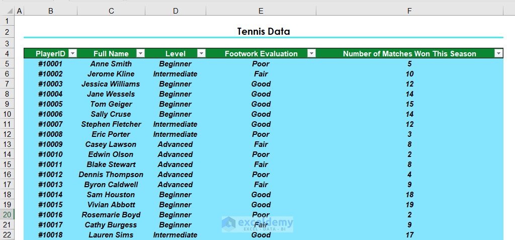
How to Create an Excel Table

Steps:

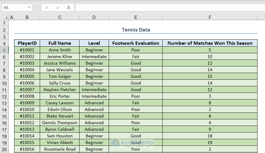
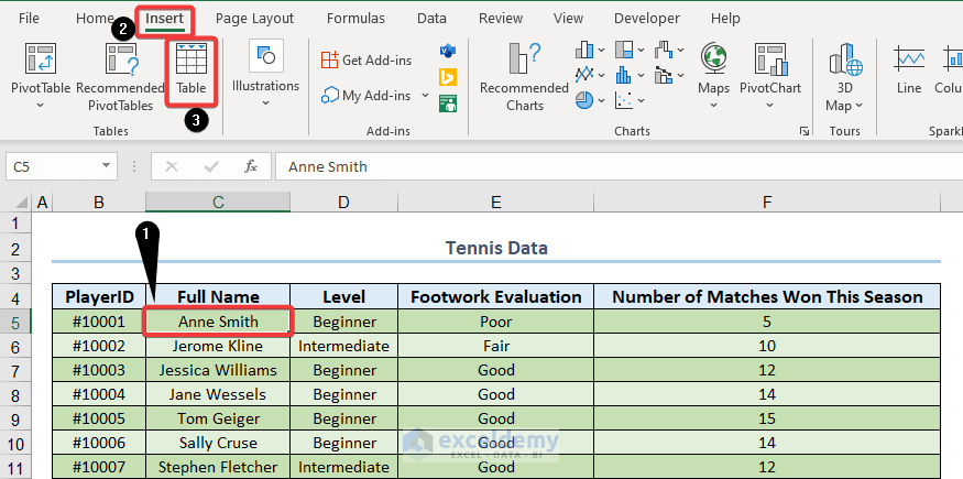
Select a cell from the data set.

A sample of Excel dataset

Go to the Insert tab and choose Table.

creating an excel table

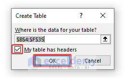
Excel will automatically pick the data for you. Check the box next to My table contains headers, then click OK.

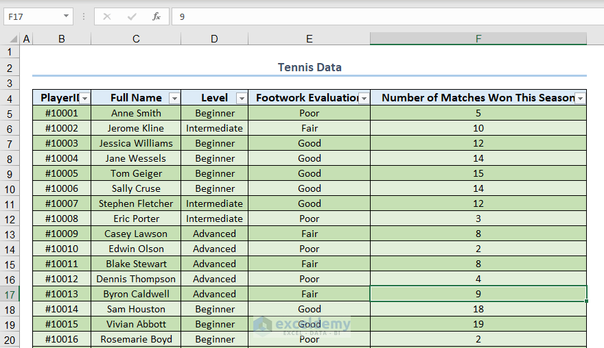
Excel will format a table.

Or,

Choose your desired dataset and click the button Ctrl + T.

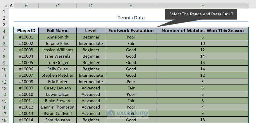
How to Make an Excel Table Look Good/Professional

Method 1 – Using Built-In Table Styles to Make a Good-Looking Excel Table

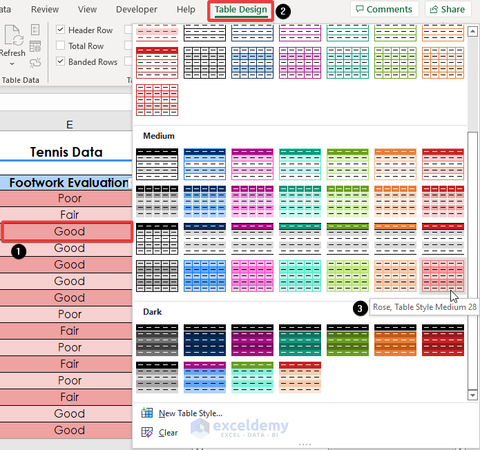
Select any cell in the table.
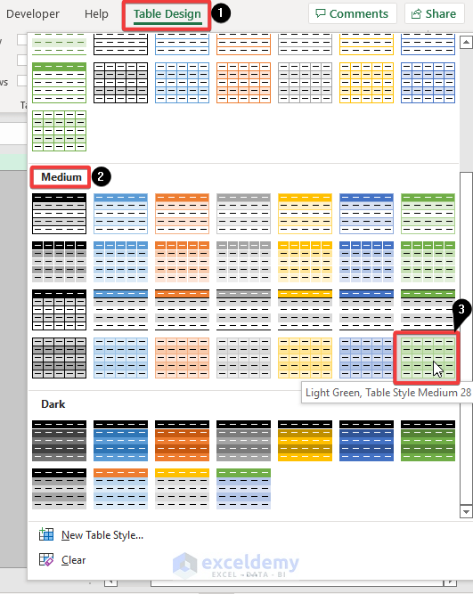
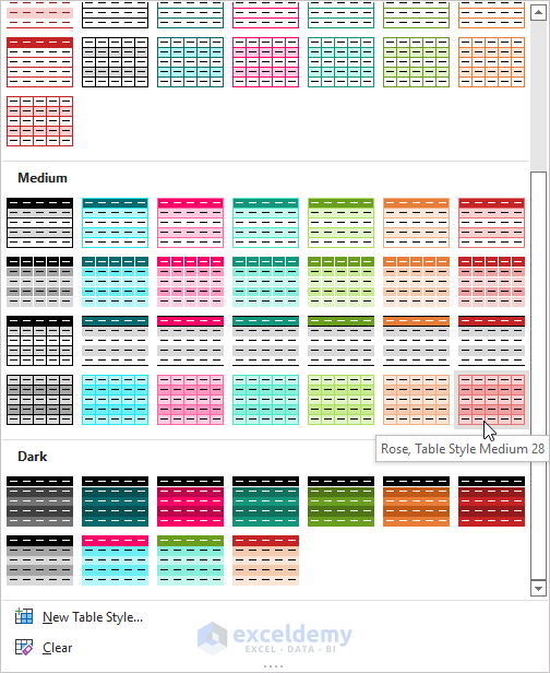
Go to Table Design and choose Table Styles, then click on the drop-down arrow.
Choose one of the built-in Table Styles available.
You can get a preview by just hovering over each style.
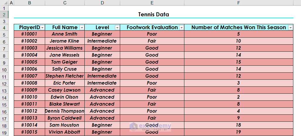
We have selected Table Style Medium 28 as shown below.

After applying this style, we get the following table.

Read More: Types of Tables in Excel: A Complete Overview

Method 2 – Changing the Workbook Theme

Go to Page Layout and select Themes, then click on the drop-down arrow below Themes and select another theme.
We chose the Slice theme.

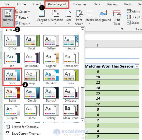
The Table Style draws its colors from the Slice theme and the effect of the change on the actual Excel Table is shown below.

Go to Table Styles to see how this affects other table styles (see Method 1).

Method 3 – Editing the Theme Color

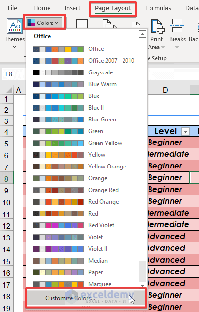
With any theme currently selected, go to Page Layout and to Themes, then click on the drop-down next to Colors.

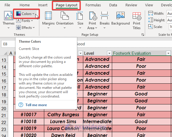
Choose the Customize Colors option.

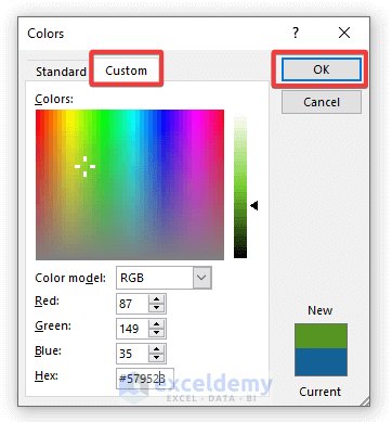
In the Create New Theme Colors dialog sox, select the drop-down arrow next to Text/Background – Dark 2 and choose More Colors.

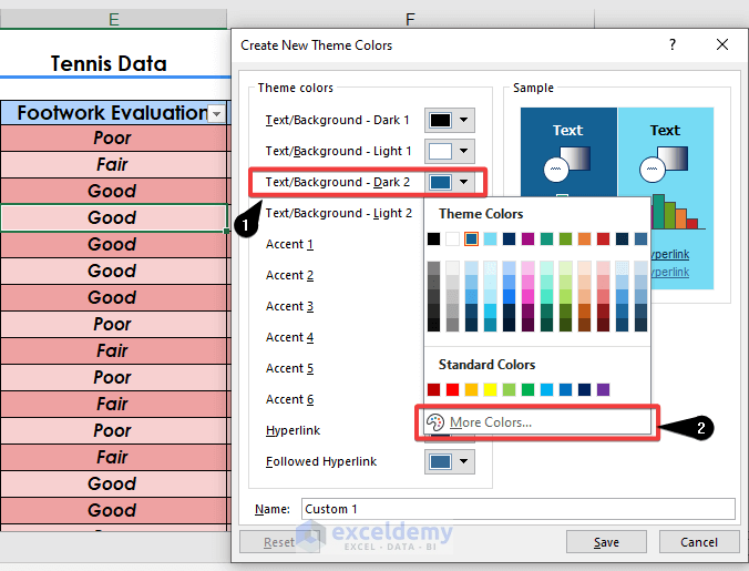
Select the Custom Tab and enter the following values: R 87, G 149, and B 35, in order to set this dark green color and click OK.

In the Create New Theme Colors dialog box, select the drop-down next to Text/Background – Light 2 and choose More Colors.

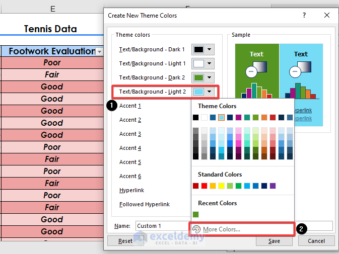
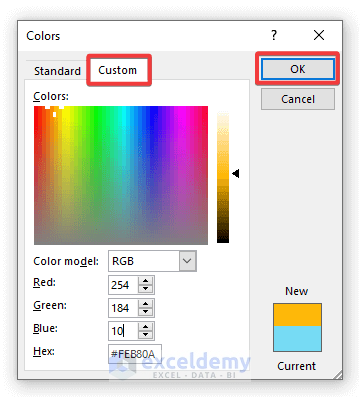
Select the Custom tab and enter the following values: R 254, G 184, and B 10, in order to set this orange color and click OK.

In the Create New Theme Colors dialog box, select the drop-down next to Accent 1 and choose More Colors.

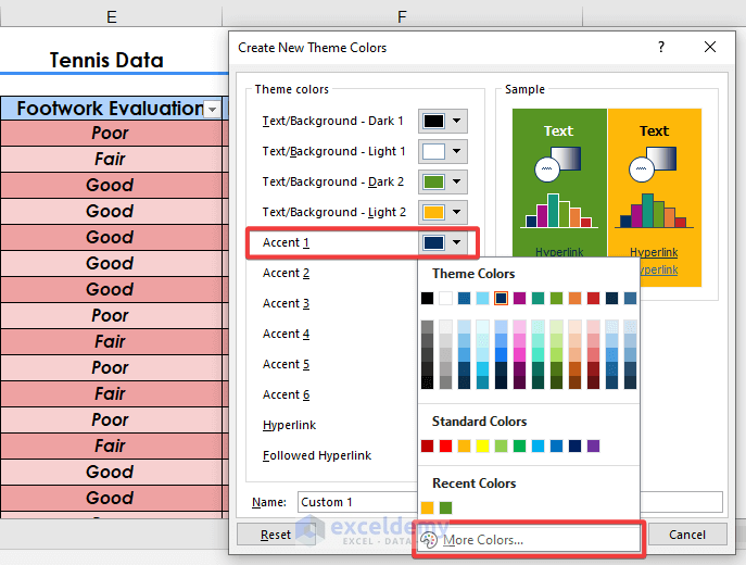
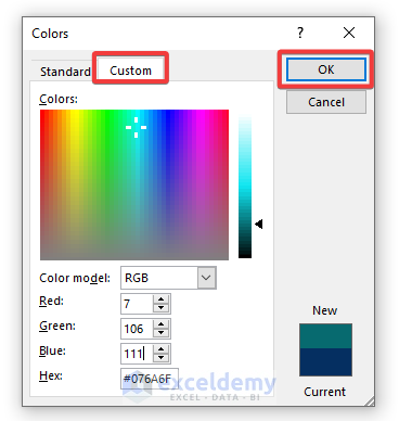
Select the Custom Tab and enter the following values: R 7, G 106, and B 111, in order to set this dark turquoise color, and click OK.

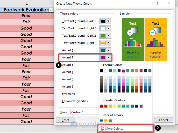
In the Create New Theme Colors dialog box, select the drop-down next to Accent 2 and choose More Colors.

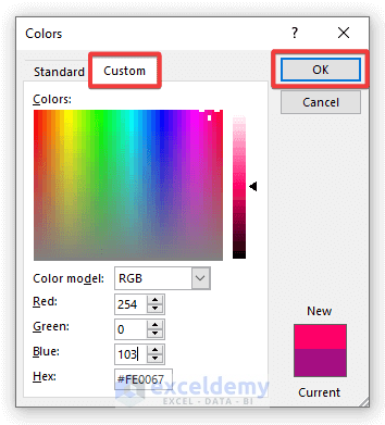
Select the Custom Tab and enter the following values: R 254, G 0, and B 103, in order to set this pink color, then click OK.

Give your new customized theme set a name and click Save.

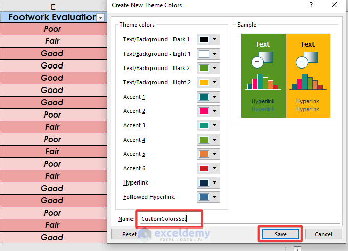
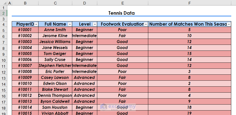
Here’s the result.

The changes will also affect other Table Styles.

Read More: Excel Table vs. Range: What Is the Difference?

Method 4 – Clearing a Style from an Excel Table

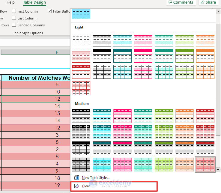
Go to Table Design and expand Table Styles.
Select Clear.

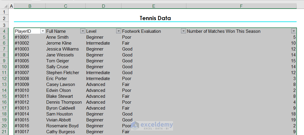
Any formatting associated with the specific table style chosen is now cleared as shown below.

Method 5 – Creating a Custom Excel Table Style

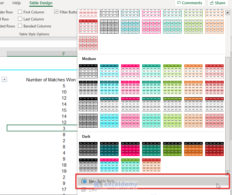
In Table Design click on the drop-down arrow next to Table Styles and select New Table Style.

You can now format individual elements of the Table using the New Table Style dialog box.

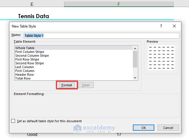
Select Whole Table and then choose Format.
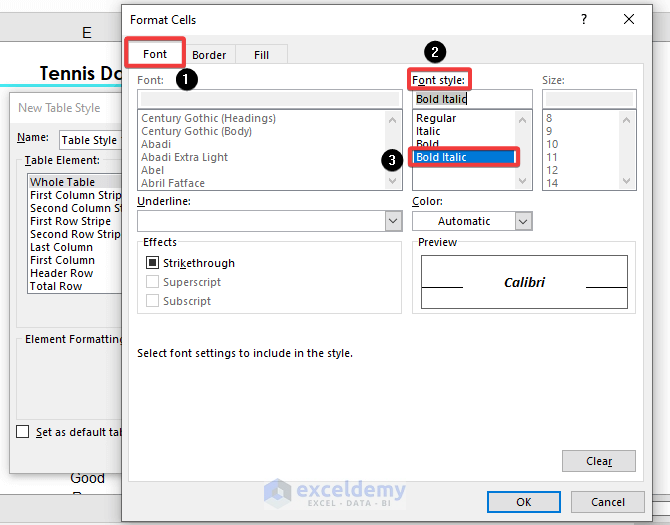
The Format Cells dialog box should appear. Choose the Font Tab, and under font style choose Bold Italic.

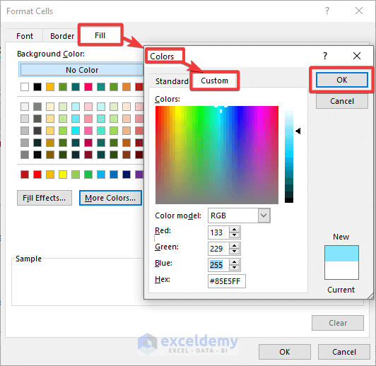
Go to the Fill tab and, under the Background Color option, choose More Colors.

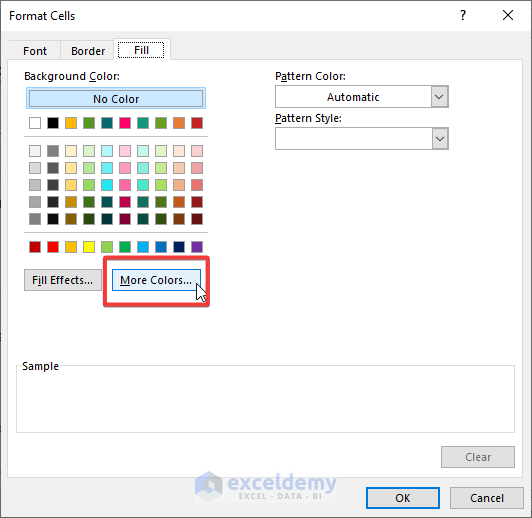
Select the Custom tab, set: R 133, G 229, and B 255 as shown below, and then click OK.

Click OK.
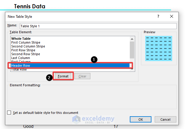
Select the Header Row element as shown below and click Format.

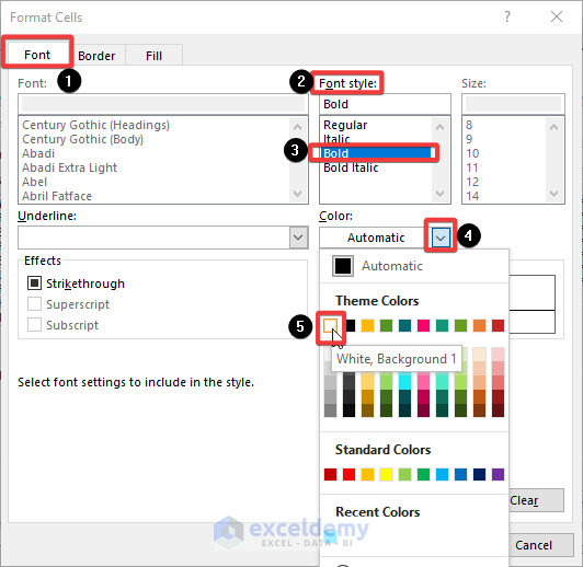
The Format Cells dialog box should appear as before. Choose the Font Tab, and under Font Style choose Bold and change the font color to White, Background 1.

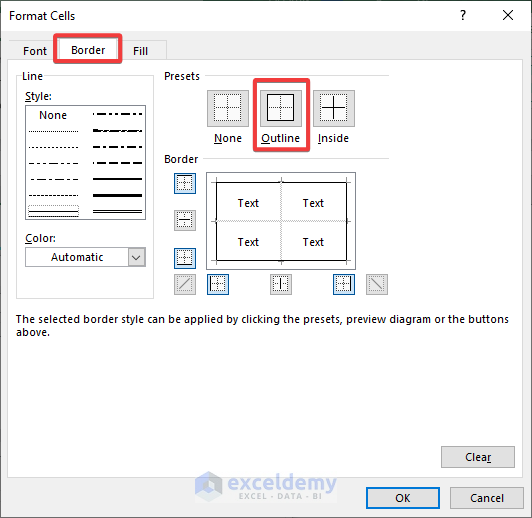
Choose the Border tab, select the thick line style, and the color: Gray – 25%, Background 2, Darker 50%.

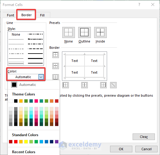
Choose Outline.

Select the Fill tab and, under Background Color, choose More Colors.

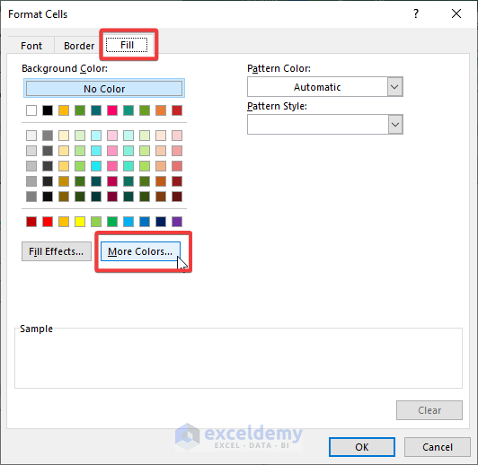
Select the Custom tab, set: R 11, G 135, and B 52 as shown below, and then click OK.

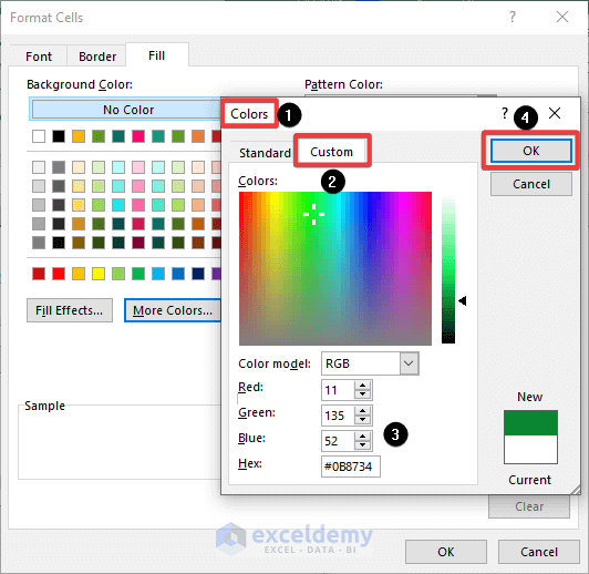
Click OK.
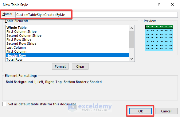
Give your new Table Style a name and check the Set as default table style for this document option to keep the changes for other tables you make.

Applying this Custom Table Style to the table results in the following look.

Read More: Navigating Excel Table

Method 6 – Adding the Total Row and Turn the Filter Button Off

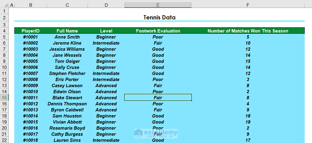
With one cell in your table selected, go to Table Design, check Total Row, and uncheck Filter Button.

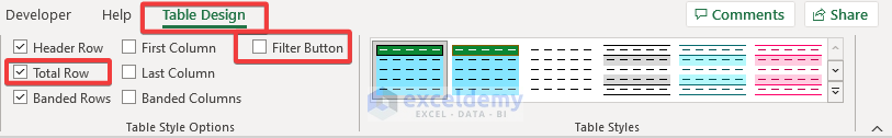
The table will have the following look.

Read More: How to Insert or Delete Rows and Columns from Excel Table

Method 7 – Inserting Slicers

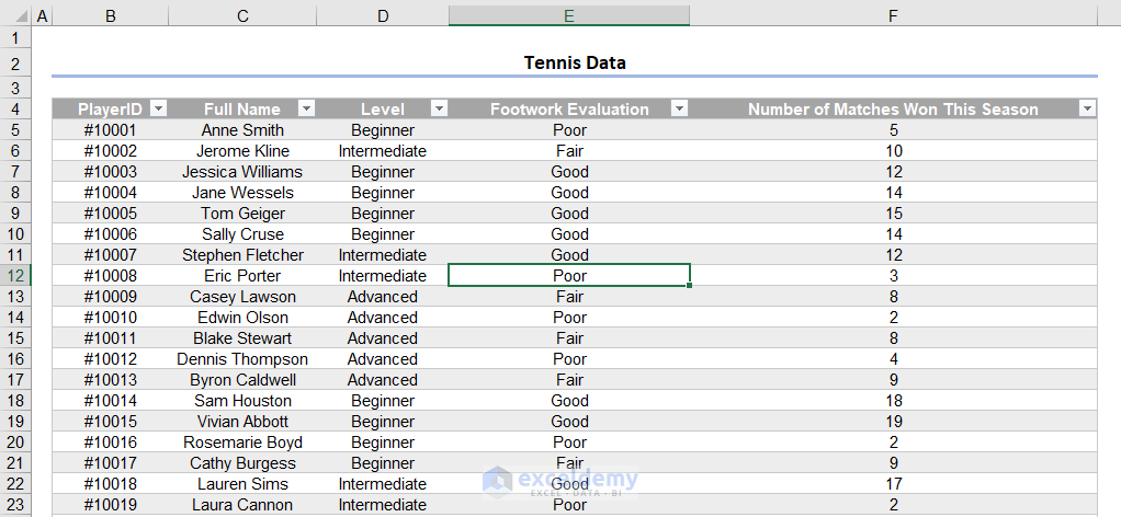
Format the table with Table Style Medium 4 (make sure the theme is the default Office theme).

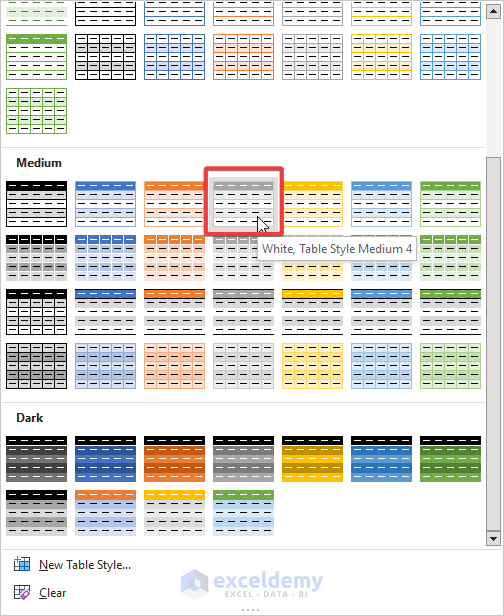
Now the entire table has the format with this style as shown below.

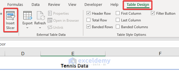
With one cell in the table selected, go to Table Design and select Insert Slicer.

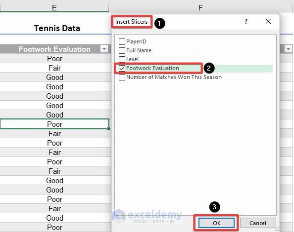
Choose one or more slicers to filter the data by. We’ll choose Footwork Evaluation as shown below and then click OK.

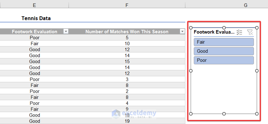
The Slicer with the default style appears as shown below.

With the slicer selected, go to Slicer Tools then to Options and choose Slicer Styles.
Select one of the default built-in styles.

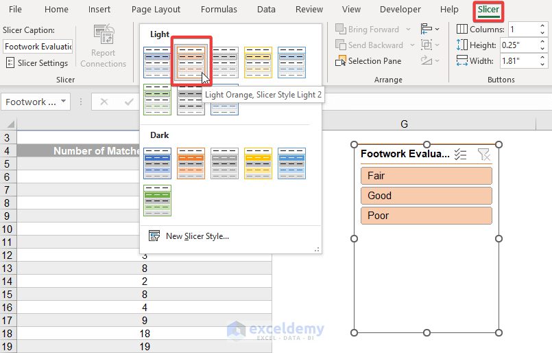
This changes the Slicer Style to the following format.
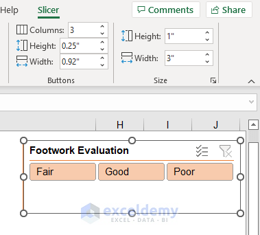
With the Slicer selected, go to Slicer Tools then to Options and select Buttons, then change the number of columns to 3.
Go to Slicer Tools then to Options and to Size, then change the height of the slicer to 1 inch and the width to 3 inches as shown below.

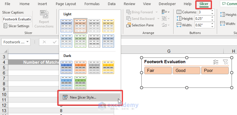
Go to Slicer Tools and select New Slicer Style as shown below.

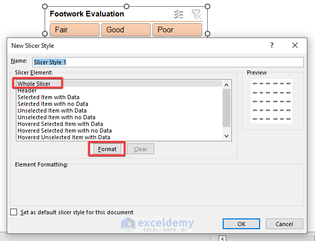
In the New Slicer Style dialog box, choose the Whole Slicer element and then click Format.

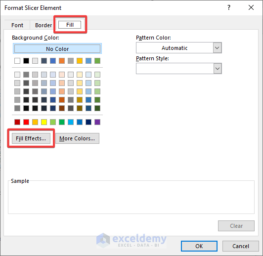
In the Fill tab, under Background Color, choose Fill Effects.

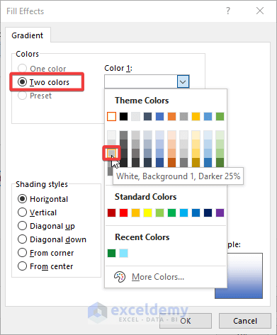
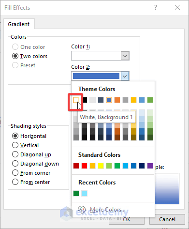
Using the Fill Effects dialog box, change Color 1 to White, Background 1, Darker 25%, and change Color 2 to White, Background 1 as shown below.

Add more colors.

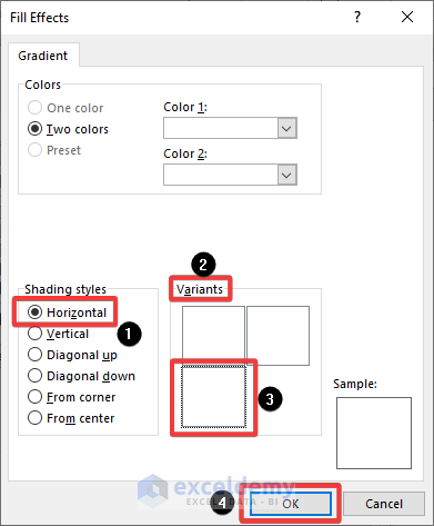
Under Shading styles, make sure Horizontal is selected and choose the third variant as shown below.

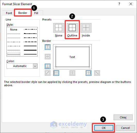
Click OK and then select the Border tab, choose the thin line style and White Background 1, Darker 35%, and then select Outline as shown below.

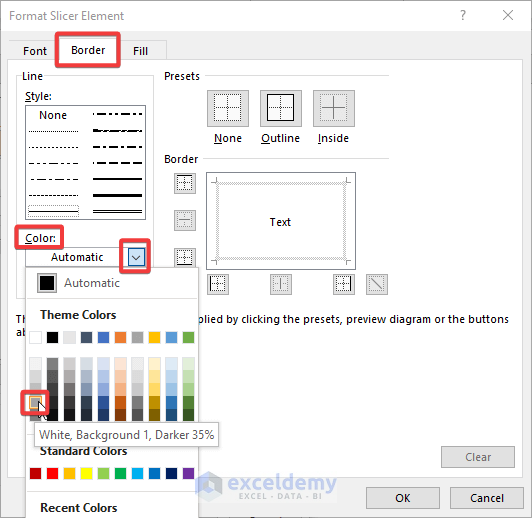
Choose a proper outline.

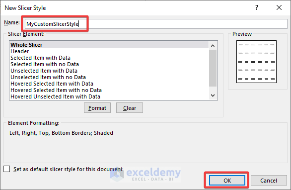
Click OK, then name your newly created Slicer Style as shown below and click OK.

Apply the new Slicer Style you just created.
Go to View and to Show, then uncheck Gridlines.

Read More: How to Convert Table to List in Excel

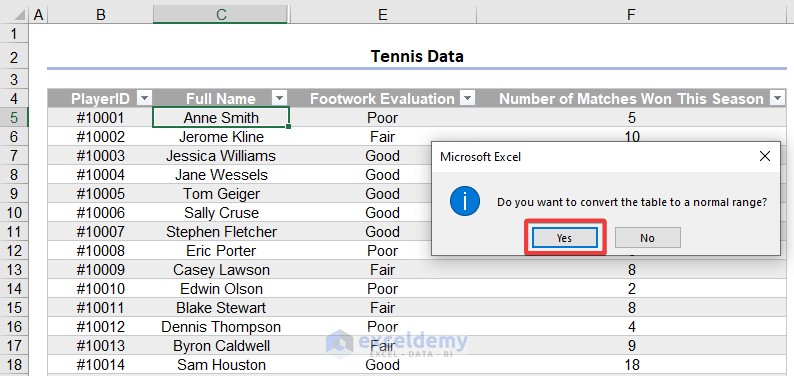
Method 8 – Converting a Table Back to a Range

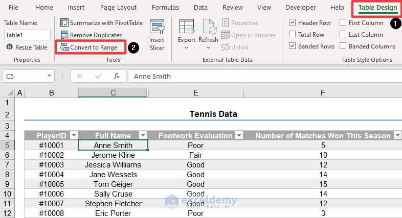
Go to Table Design and select Convert to Range.

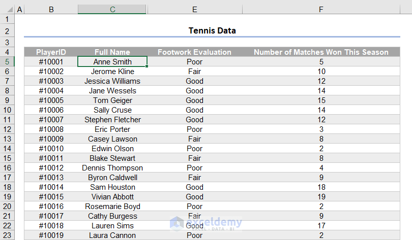
Select Yes.

The table should now be converted to a normal range but with the formatting selected still intact as shown below.

Download the Practice Workbook

Making Excel Tables Look Good.xlsx

Further Readings

<< Go Back to Edit Table | Excel Table | Learn Excel

Get FREE Advanced Excel Exercises with Solutions!

SaveSavedRemoved 0

Tags: Edit Excel Table

Taryn Nefdt

Taryn is a Microsoft Certified Professional, who has used Office Applications such as Excel and Access extensively, in her interdisciplinary academic career and work experience. She has a background in biochemistry, Geographical Information Systems (GIS), and biofuels. She enjoys showcasing the functionality of Excel in various disciplines. She has over ten years of experience using Excel and Access to create advanced integrated solutions.

2 Comments

Reply
Krishnaprasad Menon Dec 19, 2017 at 11:12 AM

Exceldemy team & its captain Mr.Kawser Ahmed is doing an excellent job by imparting knowledge on various Excel topics of importance. i like the informative & quality articles provided by Ms.Taryn. Thanks. Keep it up.
- Reply
  Kawser Dec 19, 2017 at 7:56 PM
  
  Thanks, Menon for your valuable feedback.

Leave a reply Cancel reply

Submit Excel Problem