Excel Table Formatting Problems (with Solutions)

In this article, we will discuss table formatting problems in Excel. We’ll use a simple dataset to show solutions.

Excel Table Formatting Problems: 4 Different Problems with Their Solutions

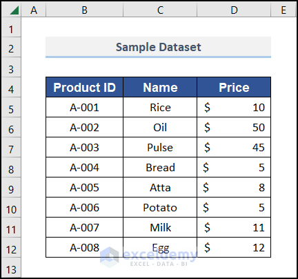
We have a dataset with Product IDs and their Prices.

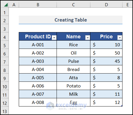
We converted the dataset into a table.

Problem 1 – Copy Formulas by Dragging with Table References in Excel Table Formatting

We want to find Prices against the Product ID. We use the INDEX function here to do that. We set 3 IDs to get the price.

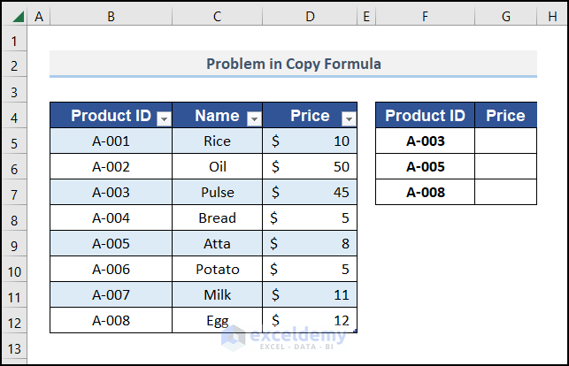
We used the following formula to get the price of the ID mentioned in cell G5.

=INDEX(Table2[Price],MATCH(F5,Table2[Product ID],0))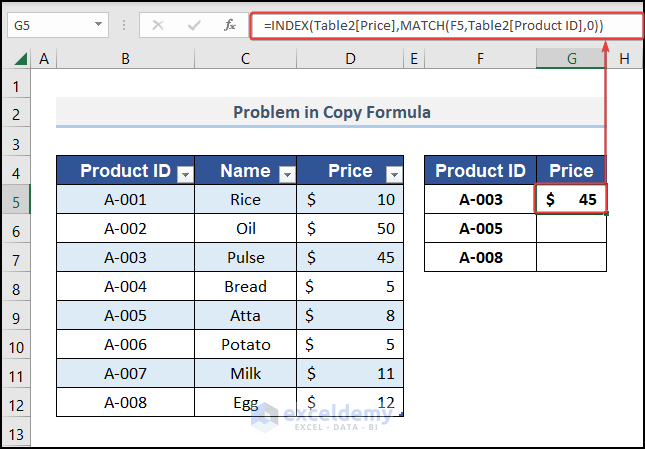

We dragged the Fill Handle icon down. We see that #N/A is showing.

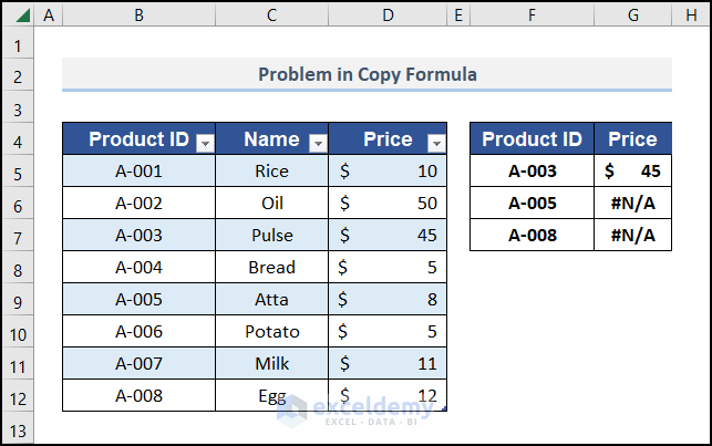
Here, the Table References are changed when dragging toward the right.

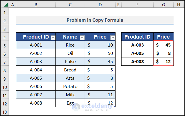
Solution:

Copy the formula from cell G5 and paste it into cells G6 and G7.

Problem 2 – Insufficient Execution of Structured Table Formatting

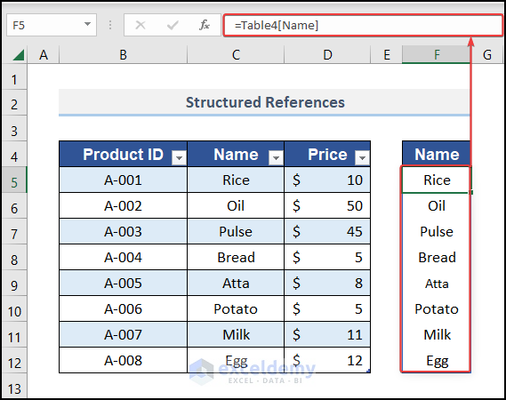
We can refer to a table column or table cell in a formula. From the formula, we noticed that it is a Structured Reference rather than a regular cell reference. Usually, we refer to any column or cell value as a reference, but here we used a table modifier reference. The @ symbol identifies a specific cell where you want to put the reference. It cannot show the entire column value rather it shows an entity. See the image for better visualization.

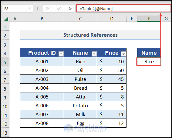
Here, the symbol in the structured formula refers to a particular cell. That is why it returns Rice instead of the whole column. Remove the @ symbol, and you will get the corresponding column where you entered the reference.

Read More: How to Extend Table in Excel

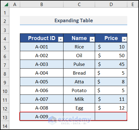
Problem 3 – Table Expansion Problem When Adding New Data in Excel

We want to add a new value to your data table. You cannot insert the value according to the table. It becomes a cell value.

We want to add a new data row. We put a value next to the cell where the table ends.

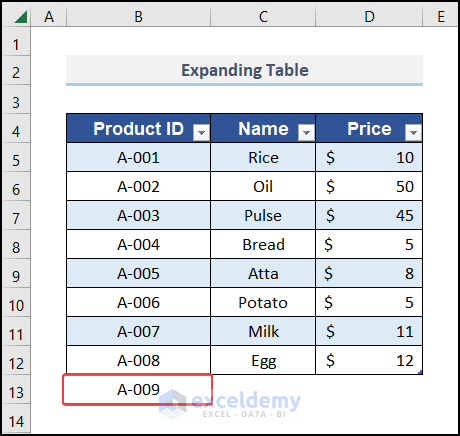
The new data is not added to the table. We can solve this by changing AutoFormat settings.

Solution:

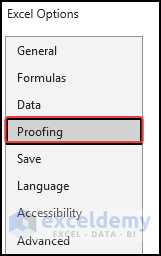
Press File, then click Option.
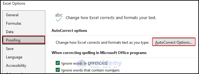
From the Excel Options window, select Proofing.

Select AutoCorrect Options.

Select AutoFormat As You Type.

Select the boxes of the last two options and hit OK.

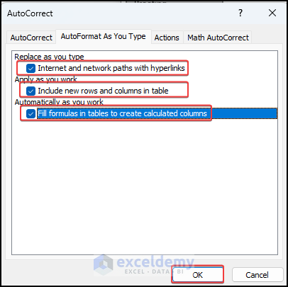
Move to cell B13 and insert any value.

The table is expanded.

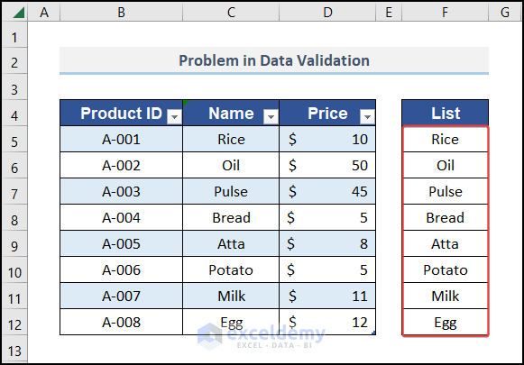
Problem 4 – Data Validation Problem in Excel Table

We made a drop-down list and used it in the Table. A column named List is added.

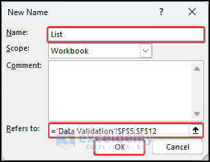
We defined a name for the new column.

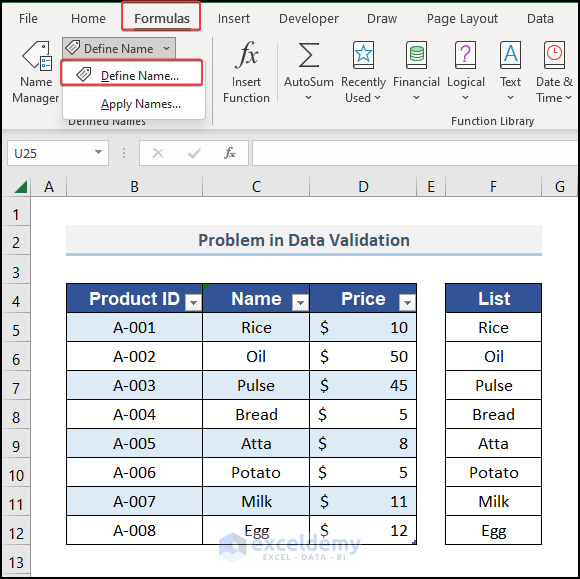
We used List for the name.

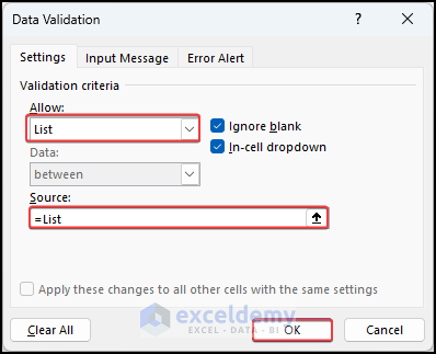
We applied Data Validation to all cells in the Name column.

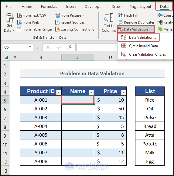
The Data Validation will source data from the named range List.

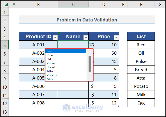
We went to the cells of the column and selected names from the drop-down.

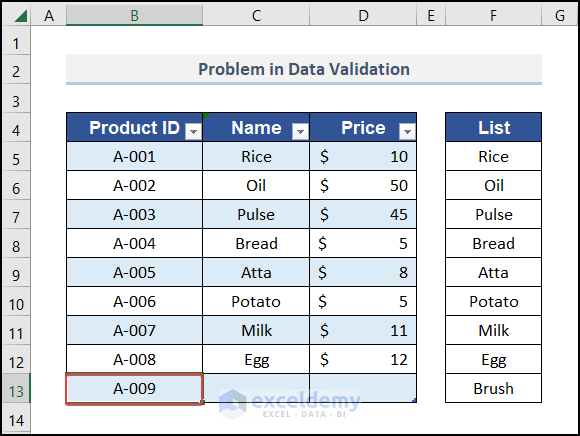
We added a new row to the table, but the drop-down list is not showing for this cell.

Solution:

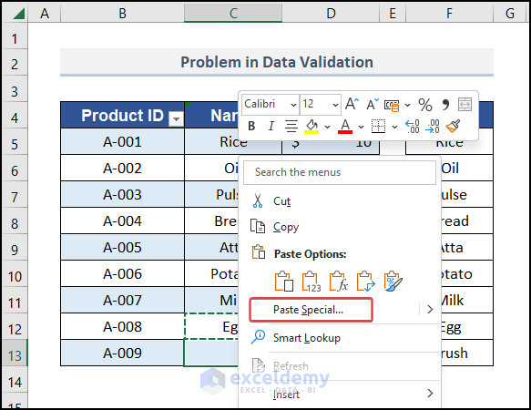
Copy any cell that contains a drop-down.
Select all the new cells.
Right-click on the selection.
Go to Paste Special.

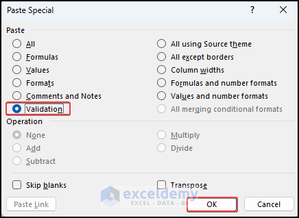
Select Validation from Paste Special.
Hit OK.

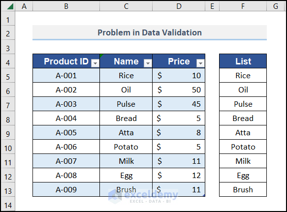
You can find that the validation-related problem has vanished.

Read More: How to Mirror Table in Excel

Some More Problems in Excel Table Formatting

In the case of protected sheets, the Table will not work properly. We can’t easily add or remove rows.
When we use a large table, our workbook will work slowly.
When we add protections to lock our formula, the table functions are lost. Specifically, it will no longer auto-expand.
When we link tables in other workbooks, the links will return a #REF! error if the source workbook is not open. By changing all links to relative cell references, we can solve this.
When we delete data from our table, the table doesn’t automatically shrink. We need to resize the table manually. We can do this with the Resize Table option or by deleting the rows.

Download the Practice Workbook

Table Formatting Problems.xlsx