Overview:
Method 1 – Deleting the Format in the Table Design Tab in Excel
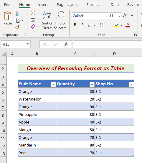
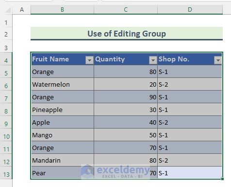
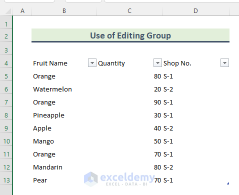
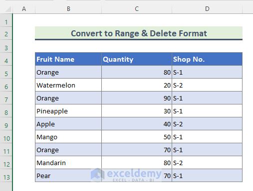
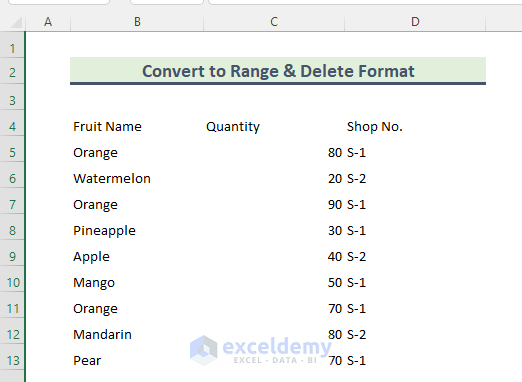
This is the sample dataset.
- To create a table, select the data and press Ctrl+T. The table will be created with default formatting.
To delete formatting:
Steps:
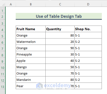
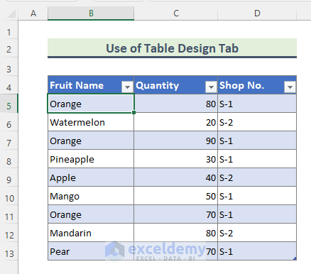
- Select any cell in the table.
- Go to Table Design.
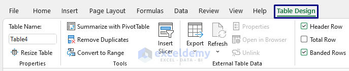
- In Table Styles, click More.
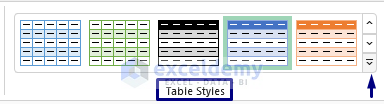
- Click Clear.
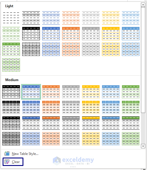
The table has no auto-generated format.

Note:
If you apply any formatting manually to the table, it can’t be removed using this method.
Read More: How to Remove Table in Excel
Method 2 – Removing Format as Table in the Editing Group in Excel
Steps:
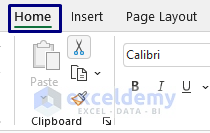
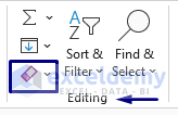
- Go to the Home tab on the Ribbon.
- Select Editing and click Clear.
- Click Clear Formats in Clear.
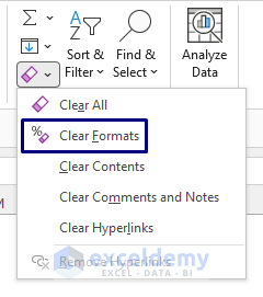
Format will be deleted.
Read More: How to Remove Table Functionality in Excel
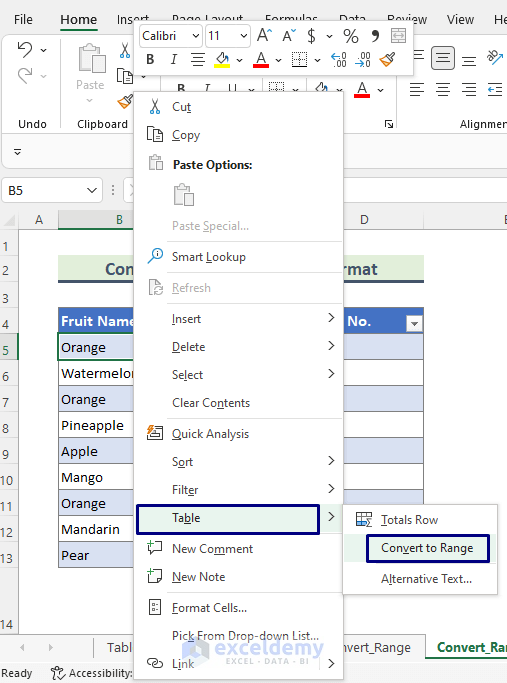
Method 3 – Convert a Table to a Range and Clear the Format in Excel
Steps:
- Select a cell in the table.
- Go to Table Design.
- Click Convert to Range in Tools.
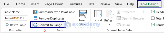
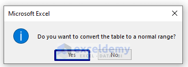
- A confirmation window will open. Click Yes.
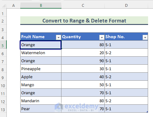
The table will be converted to a data range with formatting.
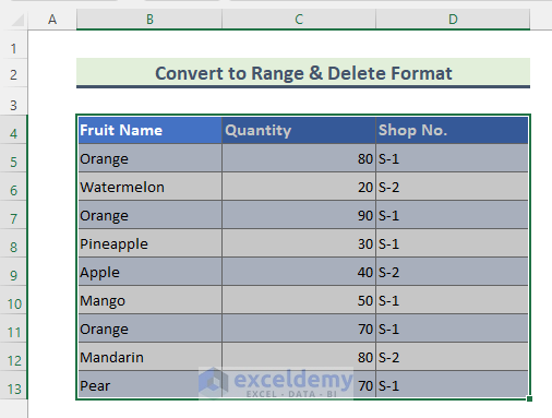
- Select the entire data range and follow the steps described in Method 2.
- Go to Home > Clear (Editing Group) > Clear Formats
This is the output.
Note:
You can also convert tables into data ranges by right-clicking a cell in the table, and in the Table option, clicking Convert to Range.
Read more: Excel Table Formatting Problems
Download the Practice Workbook
Download the practice workbook.
Further Readings
- How to Make an Excel Table Expand Automatically
- How to Use Sort and Filter with Excel Table
- How to Insert or Delete Rows and Columns from Excel Table
- How to Mirror Table in Excel
- [Fix]: Formulas Not Copying Down in Excel Table
- How to Rename a Table in Excel
- How to Extend Table in Excel
- How to Undo a Table in Excel
<< Go Back to Make an Excel Table | Excel Table | Learn Excel
Get FREE Advanced Excel Exercises with Solutions!
