We have a large Excel worksheet that contains information about several sales representatives. We want to mirror that table.
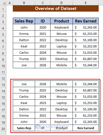
Method 1 – Use the OFFSET Function to Mirror a Table
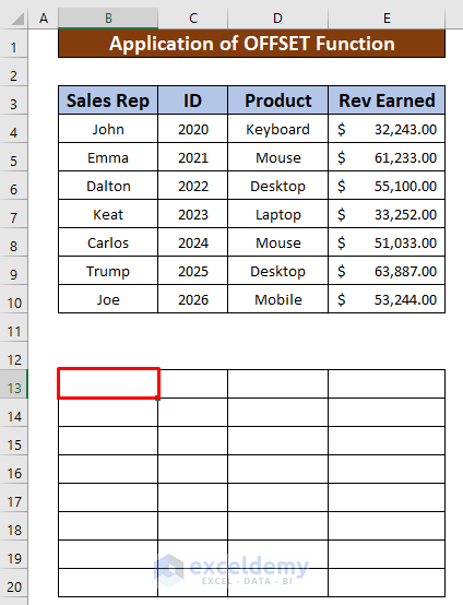
Steps:
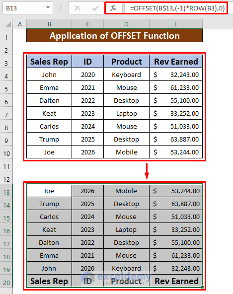
- Select cell B13.
- Use the following formula in the Formula Bar:
=OFFSET(B$13,(-1)*ROW(B3),0)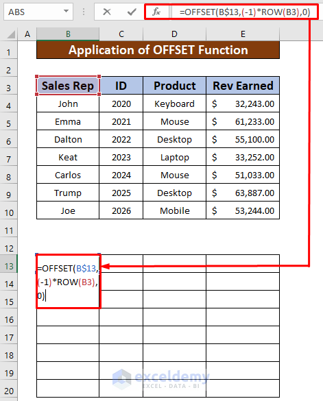
- Press Enter.
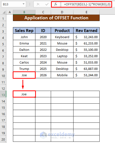
- Autofill the function to the rest of the cells horizontally.
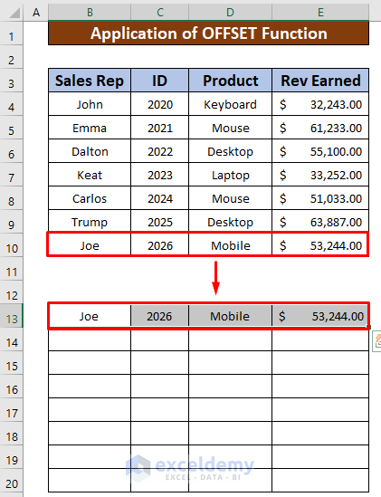
- Autofill the rows vertically.
Read More: How to Rename a Table in Excel
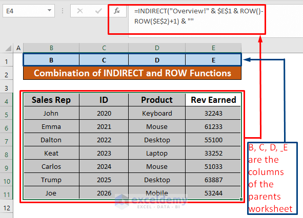
Method 2 – Combine INDIRECT and ROW Functions to Mirror a Table
Steps:
- Select cell B4.
- Insert the following formula in the Formula Bar:
=INDIRECT("Overview!" & $B$1 & ROW()-ROW($B$2)+1) & ""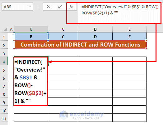
- Press Enter on your keyboard.
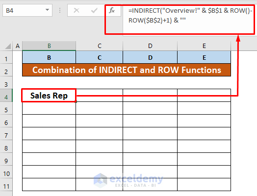
- Autofill the column.
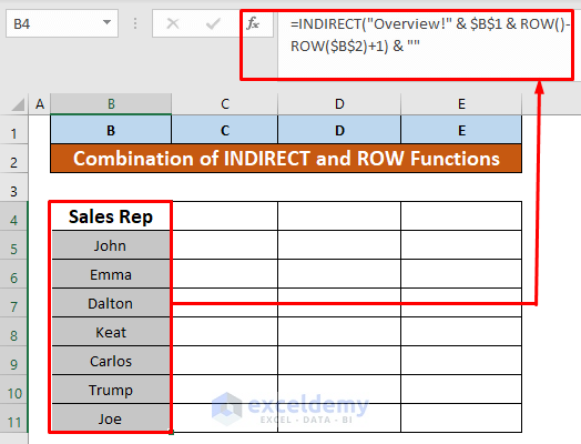
- AutoFill through the columns.
Read More: How to Extend Table in Excel
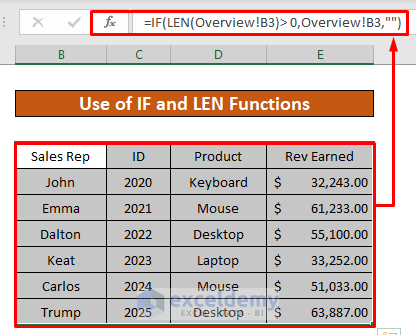
Method 3 – Merge IF and LEN Functions to Copy a Table
Steps:
- Select cell B4.
- Use the following formula in the Formula Bar:
=IF(LEN(Overview!B3)> 0,Overview!B3,"")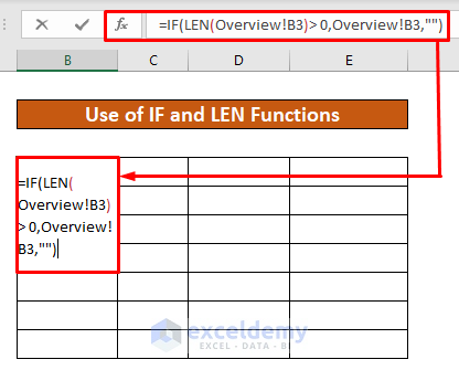
- Press Enter on your keyboard.
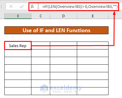
- Autofill the IF and LEN functions to the rest of the cells in that table which has been given in the screenshot.
Read More: How to Make an Excel Table Expand Automatically
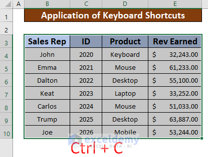
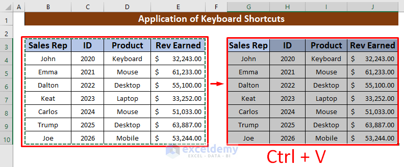
Method 4 – Apply Keyboard Shortcuts to Copy a Table in Excel
Steps:
- Select the cell range B3:E10.
- Press Ctrl + C.
- Select the destination cell.
- Press Ctrl + V to paste the copied cells.
Read More: How to Use Sort and Filter with Excel Table
Things to Remember
➜ While a value cannot be found in the referenced cell, the #N/A! error happens in Excel.
➜ #DIV/0! error happens when a value is divided by zero (0) or the cell reference is blank.
Download the Practice Workbook
Related Articles
- How to Insert or Delete Rows and Columns from Excel Table
- How to Remove Format As Table in Excel
- Excel Table Formatting Problems
- [Fix]: Formulas Not Copying Down in Excel Table
- How to Remove Table Functionality in Excel
- How to Remove Table in Excel
- How to Undo a Table in Excel
<< Go Back to Edit Table | Excel Table | Learn Excel
Get FREE Advanced Excel Exercises with Solutions!
