When you have a large table as a dataset then most of the time, you may need to Sort and Filter in Excel. In this post, I will discuss how you can Sort and Filter the data of a table in Excel.
Use Sort and Filter with Excel Table: 4 Methods
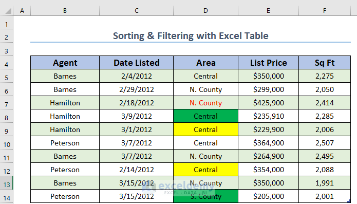
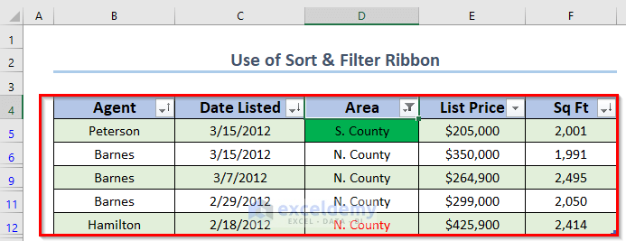
Here, I’m going to explain 3 easy methods of how to Sort and Filter with an Excel table. For your better understanding, I will use a sample dataset that contains the data of a real estate company. The dataset is given below.
1. Inserting Table to Apply Sort and Filter in Excel
You can use the features of an Excel table to Sort and Filter the data. Here, I will show you how to insert a table and how to sort and filter your data.
Steps:
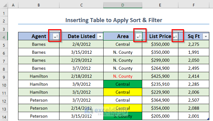
- First, you must select the data. Here, I have selected the range B4:F14.
- Next, from the Insert tab >> select the Table feature.
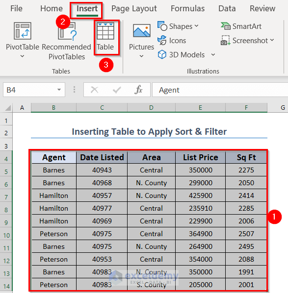
Now, a dialog box of Create Table will appear.
- Next, select the data for your table. Which will be auto-selected.
- Make sure that “My table has headers” is marked.
- Then, press OK.

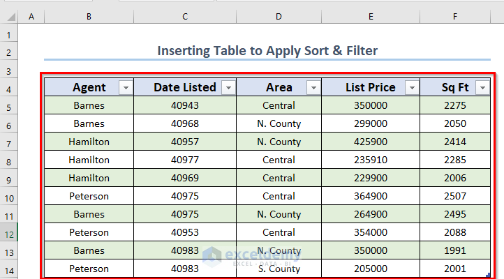
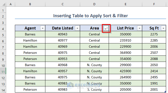
At this time, you will see the following table. As you can see, each item in the Header Row of the table contains a drop-down arrow. This drop-down arrow is known as the “Filter” button.
Now, if you click on the Filter button, you will see many types of Sorting and Filtering options.
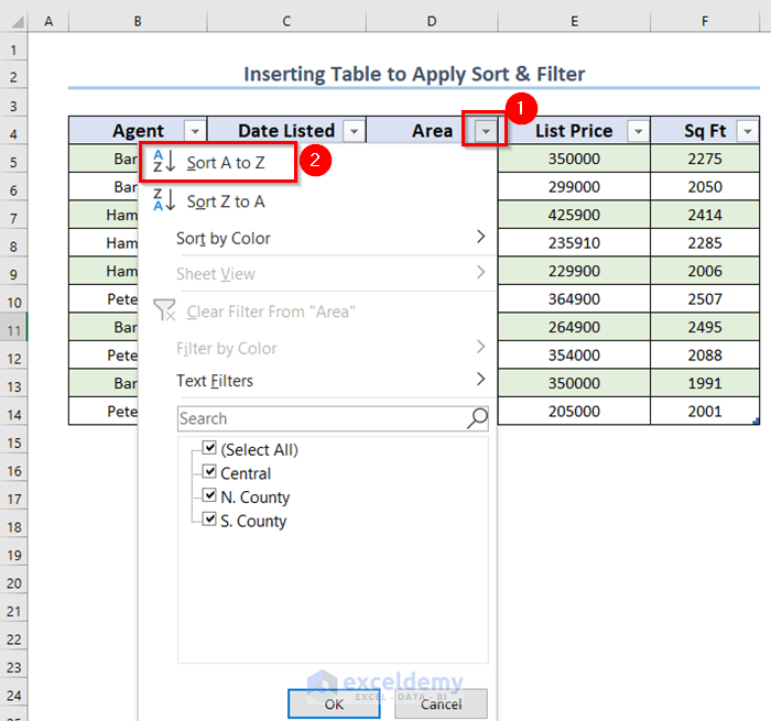
Basically, Sorting means rearranging the rows based on some criteria. For example, you may want to sort a column in alphabetical order. Now, say I want to sort this Area column in alphabetical order.
- So, click on the Filter button of the Area column. Here, you can see three sorting options: Sort A to Z, Sort Z to A, and Sort by Color.
- Then, I click on Sort A to Z.
At this time, you get a little up arrow beside the Filter button to let you know that you have sorted this column from a lower alphabetical letter to a higher alphabetical letter.
- Now click on the “List Price” column’s Filter button. Where the “List Price” column holds numbers. Thus, you see the sorting options have been changed. So, sorting options actually depend on the contents of a column.
- Then, I click on the “Sort Smallest to Largest” option. So, I sorted the column in ascending order.

At this time, you can see a little up arrow with the Filter button to let you know that you have sorted the “List Price” column in ascending order.

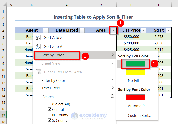
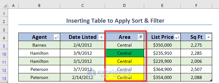
Now, I want to show how you can sort a column using background or text color. Here, you cannot sort a column using that default table background color or table default text color.
Only when you have applied different colors in cells or text by yourself, then you can sort a column using a background color or text color.
Here, for your better understanding, I have applied some background color in some cells and used some text color in some text in this column.

- Then, click on the Filter button in the Area column again >> move your mouse on Sort by Color.
At this time, a sub-menu appears. In addition, you can choose “Sort by Cell Color” or “Sort by Font Color”. As you can see, “Sort by Cell Color” has three options for this Column: Green color, Yellow Color, and No Fill color. Again, Sort by Font Color has also three color options: The Red Font color, and the Automatic Font color. Also, there is another option Custom Sort which I will discuss later.
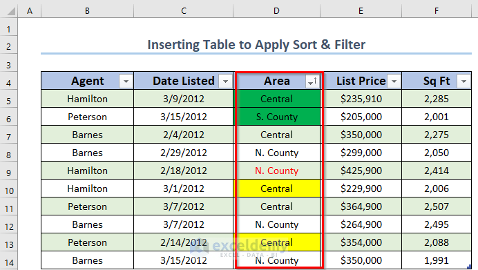
- Here, from the Sort by Cell Color option >> I selected Green color.
Subsequently, you will see the following result.
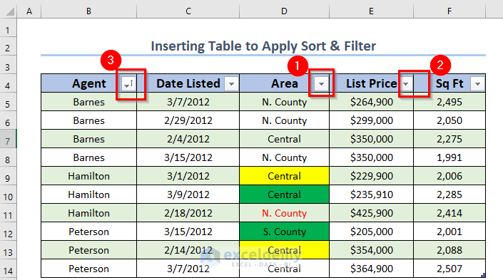
Now, let’s see how you can sort multiple columns.
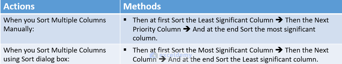
Actually, you can sort multiple columns in two ways. For example, I want to sort three Columns: Agent, Area, and List Price. When you sort multiple columns, remember one important thing: First, sort the least significant column, then sort the next priority column, and at the end, sort the most significant column.
In my case, say my least significant column is the Area column, then the List Price column, and the most significant column is the Agent column.
- So first of all, I will sort the Area column, click on the Filter button and choose the “Sort A to Z” option.
- Then, sort the List Price column, click on the Filter button, and choose the “Sort Smallest to Largest” option.
- Finally, sort the Agent column, in the Filter button, choose the “Sort A to Z” option.
This is how you can sort multiple columns.
Furthermore, there is another way you can sort multiple columns.
- Firstly, click on any Filter button.
- Secondly, move your Mouse pointer over the “Sort by Color” option.
- After that, click on the Custom Sort feature.

At this time, a dialog box named Sort appears. I want to sort a total of three columns, and in the dialog box, you can sort only one column. So, I have to add two more levels.
- Firstly, I add two more levels by clicking twice on the “Add Level” button.
In the Sort dialog box, the most significant column comes first, then the next significant column, and finally, the least significant column. Here, my most significant column was the “Agent” column, then the “List Price” column and the least significant column was the “Area” column.
- Secondly, I select Agent in the Sort by drop-down.
- Thirdly, I choose Sort on Values. Here, you can sort on Values, Cell Color, Font Color, and Cell Icon.
- Fourthly, choose the Order as A to Z. Here, to get more options click on the drop-down, Z to A, and “Custom Lists” options are there. Again, click on the Custom Lists option to open the Custom Lists dialog box.
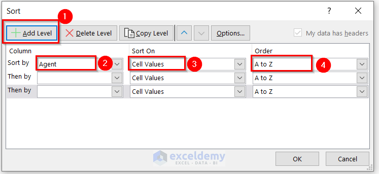
- Then, choose the List Price in the Then by box >> choose the Order as Largest to Smallest.
- Finally, select the Area column in the Then by box >> then keep unchanged the Order as A to Z.
- Subsequently, you must press OK.

In addition, you can raise your level, you can lower your level. Just select the Level, click on this Up arrow, and again click on the Down arrow. Furthermore, you can copy the level and you can delete the level. To do that, you have to click on the Options button. At that time, the Sort Options dialog box appears with More Options. Moreover, you can make your sorting Case Sensitive, and you can change the Orientation.

Lastly, you will get the sorted three columns according to the criteria.
Now, let’s now discuss how you can filter a table.
Actually, Filtering means displaying only those rows that meet certain conditions. The other rows will be hidden. For example, in this Real Estate table, you might be interested to see only the Central Area data. Apart from this, to do that filtering, you may follow the given steps.
- Firstly, click on the Filter button beside the Area column
- Secondly, unmark the Select All option.
- Thirdly, select the Central option.
- Finally, press OK.
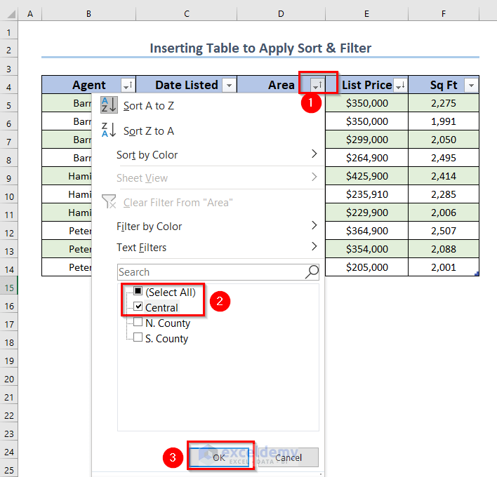
At this time, you will see that only the Central Area-related data is available on the table now. Also, notice that some row numbers are missing; they are actually hidden. Besides, notice that the Filter button of this column is now showing a different graphic which means that I have filtered this column.
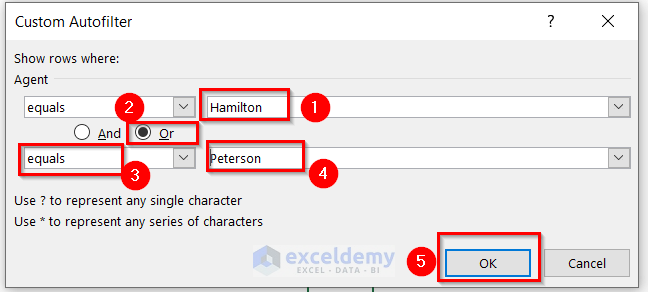
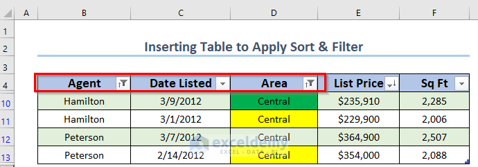
As well as that complex filtering is also possible. In addition to this, let’s assume I want to see only Hamilton and Peterson in the Agent Column and only N. County in the Area column.
- Firstly, put your mouse cursor on the Filter button beside the Agent column.
- Next, choose the “Text Filters” option. At this time, a sub-menu appears, and so many options are here. Equals, Does Not Equal, Begins With, Ends With, Contains, Does Not Contain, and Custom Filter. Dig them out by yourself and solve the homework on this topic.
- Lastly, I click on Custom Filter.

Subsequently, a Custom AutoFilter dialog box appears.
This Filtering will show rows where Agent is Equals. Furthermore, you can change it by clicking on the drop-down where you will see so many options: equals, does not equal, is greater than, is greater than or equal to, and so many others.
- Now, I select Hamilton beside the 1st equals box.
- Then, I select Or and then again equals, and then Peterson.
- Lastly, I click OK.
Last but not least, you will see only Hamilton and Peterson as agents, as shown on the table now.

In the same way, you can filter a number of columns. When you use more filtering, the total updated Rows of the table will be visible.
- Similarly, click on the Filter button beside the Area column
- Then, unmark the Select All option and then select the N. County option.
- Subsequently, press OK.
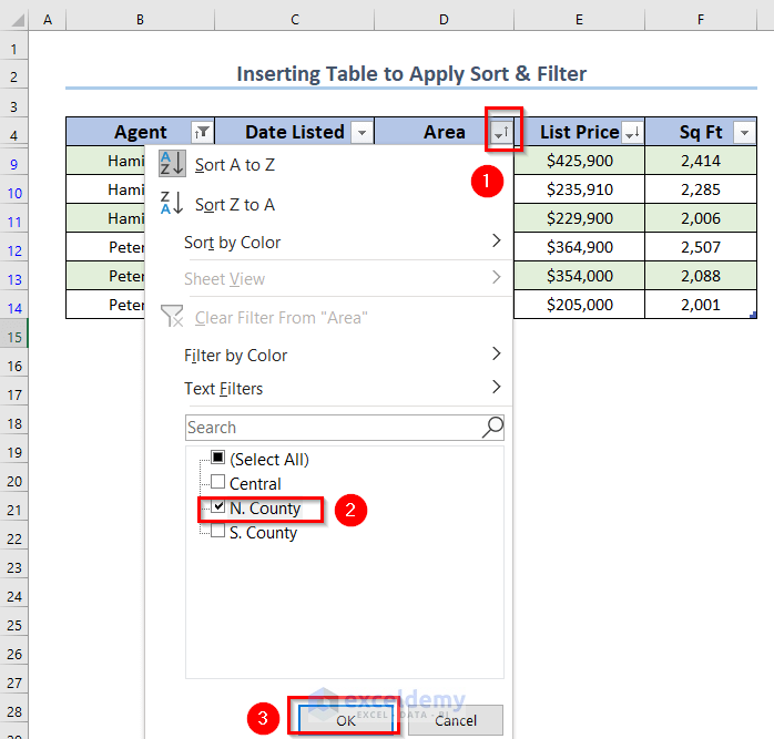
Lastly, you will see two filtered columns.
Read More: How to Rename a Table in Excel
2. Use of Context Menu Bar to Sort and Filter with Excel Table
You can use the Context Menu Bar to sort and filter an Excel table. At first, I will do the sorting.
- Firstly, select any column that you want to sort. Here, I have selected B4.
- Next, right-click on the B4 cell.
- Then, from the Context Menu Bar >> choose Sort >> then select Sort A to Z. Here, you can sort according to your preferred way.
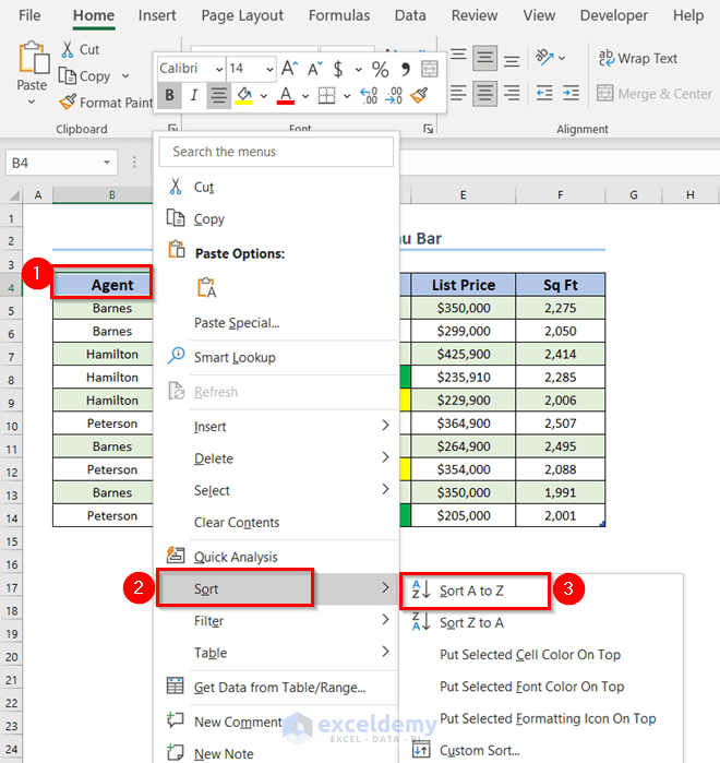
At this time, you will see the following sorted table.

Similarly, I will do filtering.
- First, select any cell that you want to sort. Here, I have selected D10.
- Next, right-click on the D10 cell.
- Then, from the Context Menu Bar >> choose Filter >> then select Filter by Selected Cell’s Color. Here, you can filter according to your preferred way.
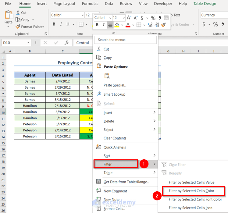
Lastly, you will see the following sorted & filtered table.

Read More: How to Extend Table in Excel
3. Employing Sort & Filter Command
Here, you can employ the Sort & Filter command to do sorting and filtering in Excel.
- First, select a cell that you want to sort or filter. Here, I have selected B4.
- Next, from the Home tab >> go to the Editing feature.
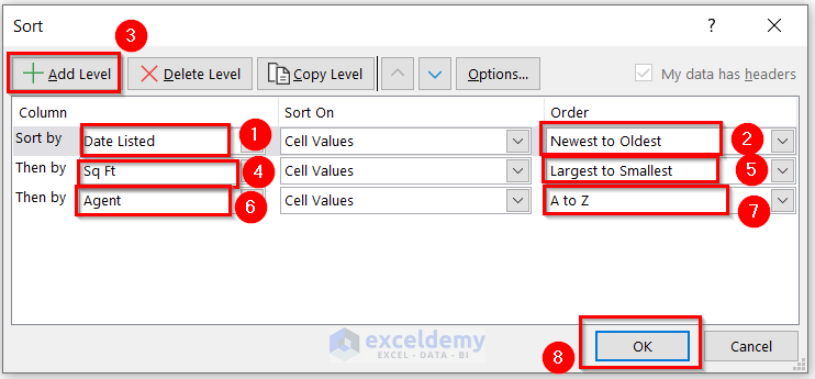
- Then, from the Sort & Filter command >> choose the Custom Sort option.

At this time, a dialog box named Sort will appear.
- Firstly, choose Date Listed as Sort by and Order as Newest to Oldest.
- Secondly, click twice on the Add Level option.
- Thirdly, choose Sq Ft as Sort by and Order as Largest to Smallest.
- Similarly, choose Agent as Sort by and Order as A to Z.
In the Sort dialog box, the most significant column comes first, then the next significant column, and finally, the least significant column. Here, my most significant column was the “Date Listed” column, then the “Sq Ft” column and the least significant column was the “Agent” column.
- Lastly, press OK.
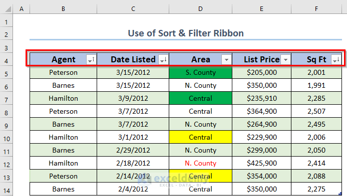
Finally, you will see the following sorted table.
Apart from this, to do that filtering, you may follow the given steps.
- First, click on the Filter button beside the Area column
- Next, unmark the Select All option.
- Then, select the N. County and S. County options.
- Lastly, press OK.

Lastly, you will see the following sorted & filtered table.
Read More: How to Mirror Table in Excel
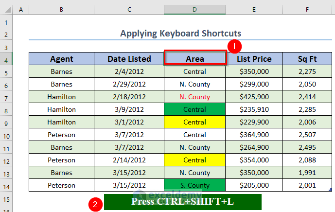
4. Applying Keyboard Shortcuts to Sort and Filter Excel Table
As well as you can apply the Keyboard Shortcuts to bring the Filter button.
- First, select any column that you want to sort. Here, I have selected D4.
- Next, press CTRL+SHIFT+L.
After that, you will see the Filter button.
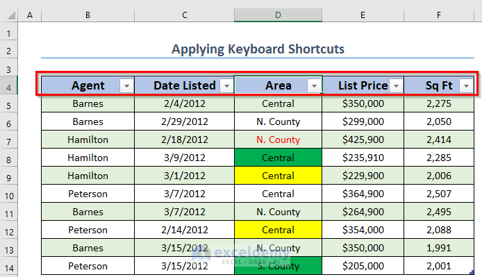
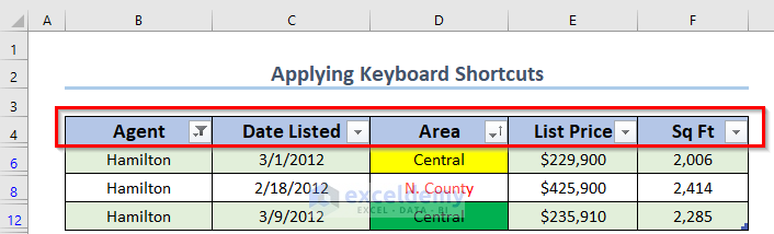
Here, you may follow method-1 to do sorting and filtering. Below, I have attached a sorted and filtered table by following the previous methods.
Read More: How to Make an Excel Table Expand Automatically
Things to Remember
- Here, to remove filtering for a column, click on the Filter button and select Clear Filter from that column.
- Furthermore, if you’ve filtered multiple columns and you want to remove all the filtering at once, then you need to click on the Sort & Filter drop-down in the Home ribbon and then select the Clear command from the list.
- Moreover, you can apply keyboard shortcuts CTRL+SHIFT+L to remove the Filter button.
Download Practice Workbook
You can download the practice workbook from here:
Conclusion
I hope you found this article helpful. Here, I have explained 4 suitable methods to use Sort and Filter with Excel Table. Please, drop comments, suggestions, or queries if you have any in the comment section below.
Related Articles
- How to Insert or Delete Rows and Columns from Excel Table
- How to Remove Format As Table in Excel
- Excel Table Formatting Problems
- [Fix]: Formulas Not Copying Down in Excel Table
- How to Remove Table Functionality in Excel
- How to Remove Table in Excel
- How to Undo a Table in Excel
<< Go Back to Excel Table | Learn Excel
Get FREE Advanced Excel Exercises with Solutions!
