Method 1 – Using PivotTable and PivotChart Wizard to Convert a Table to a List in Excel
- Introduction to the Dataset:
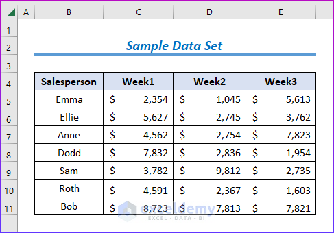
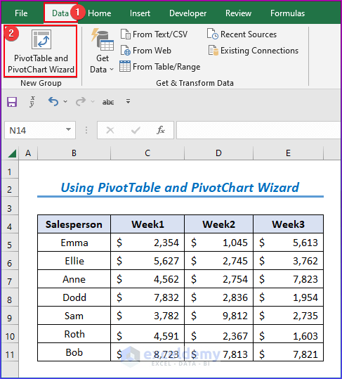
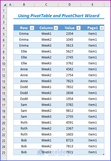
- You have a dataset containing sales data for different salespersons over three weeks.
- Objective:
- Create a list with the headings of weeks in one column and the sales amounts in another column.
- Steps:
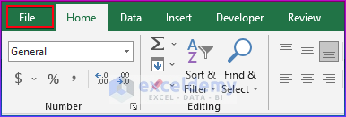
- Click on the File tab to access different options.
-
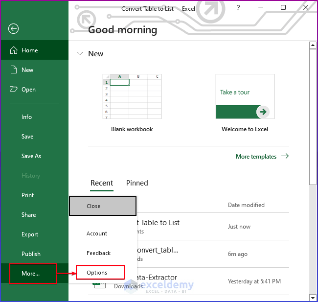
- Click on Options.
-
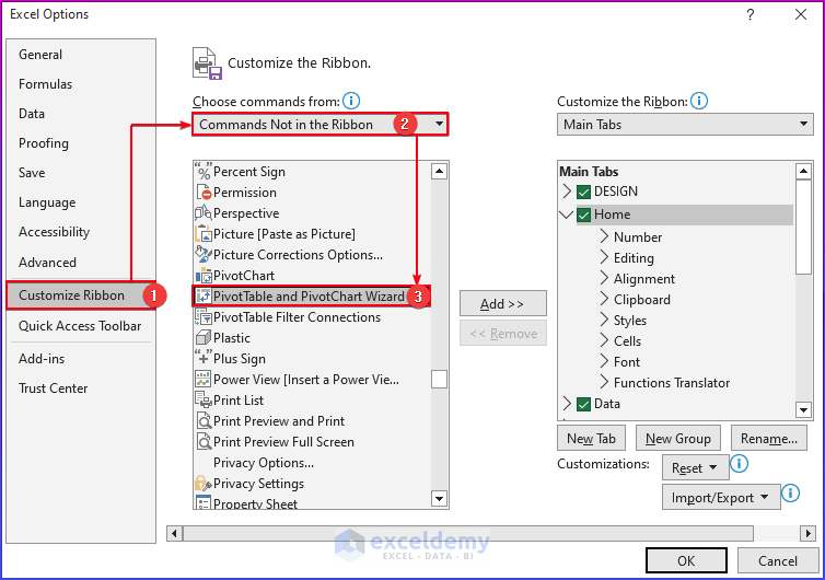
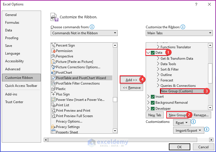
- In the Excel Options window, navigate to Customize Ribbon, select Commands Not in the Ribbon and click on PivotTable and PivotChart Wizard.
-
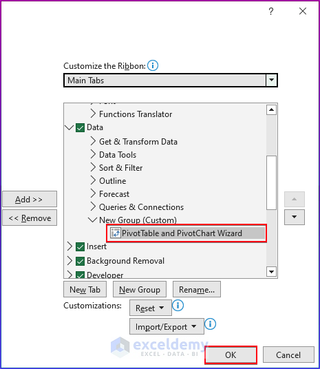
- Click Add to include this option in the top menu bar.
-
- Go to Data and select PivotTable and PivotChart Wizard.
-
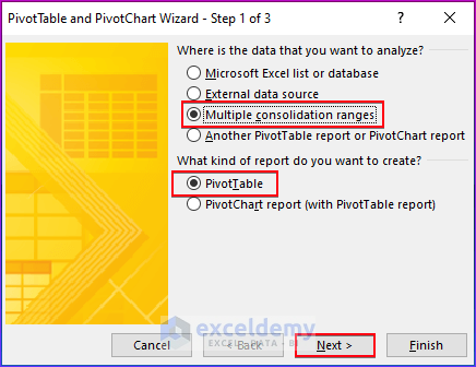
- A dialog box will appear.
-
- Select both Multiple consolidation ranges and PivotTable.
- Click Next.
-
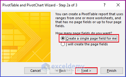
- Choose the radio button labeled Create a single page field for me and click Next.
-
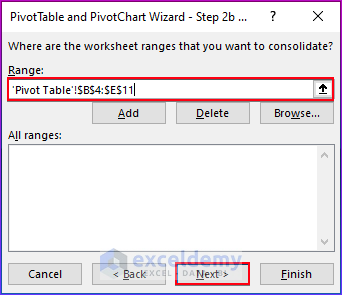
- Select the data range and click Next.
-
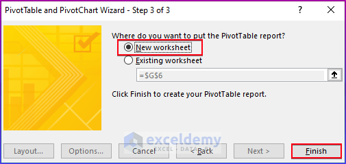
- Choose your desired worksheet (e.g., New worksheet) and click Finish.
- The PivotTable Fields will appear on the right side of your Excel window.
-
- Deselect the Row and Column options.
- Double-click on Sum of Value.
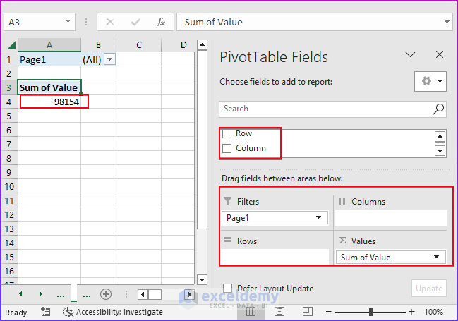
- You’ll find your desired list in a new sheet.
Read More: Types of Tables in Excel: A Complete Overview
Method 2 – Using Power Query to Convert an Excel Table to a List
Power Query is a powerful tool that simplifies the process of collecting data from various sources and organizing it into a usable format within an Excel sheet. In this method, we’ll use Power Query to convert an Excel table into a list.
Here are the steps:
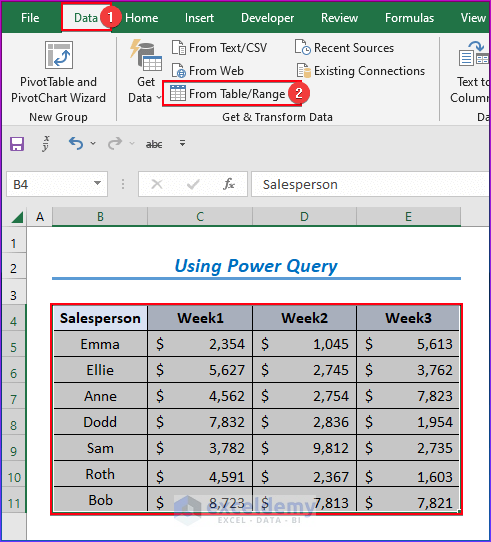
- Select the data range (the table) that you want to convert to a list.
- Click on the Data tab in Excel.
- Choose From Table/Range from the options.
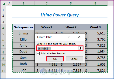
- A dialog box named Create Table will appear.
- Simply press OK to proceed.
- You’ll now see the Power Query Editor window.
- Hold down the Ctrl key and use your mouse to select the three columns representing the weeks from this window.
- Click on Transform in the Power Query Editor.
- Select Unpivot Columns.
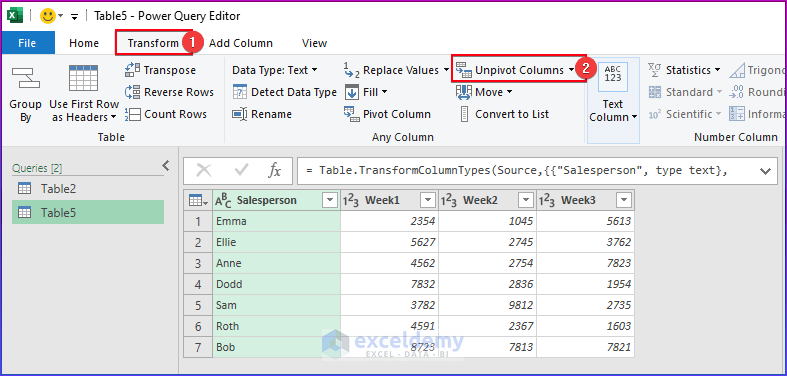
- This action will transform the columns into rows, creating a list-like structure.
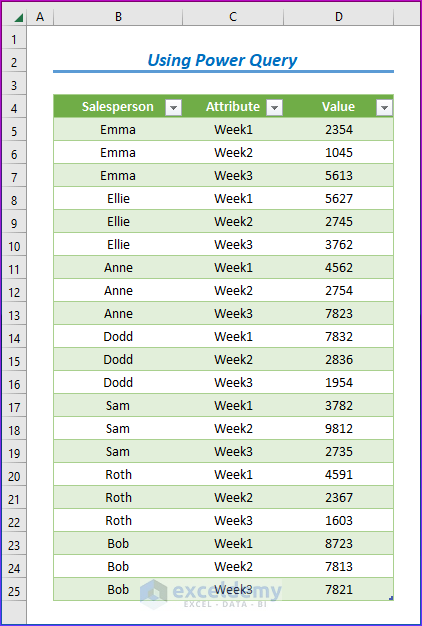
- After making the necessary transformations, click Close & Load.
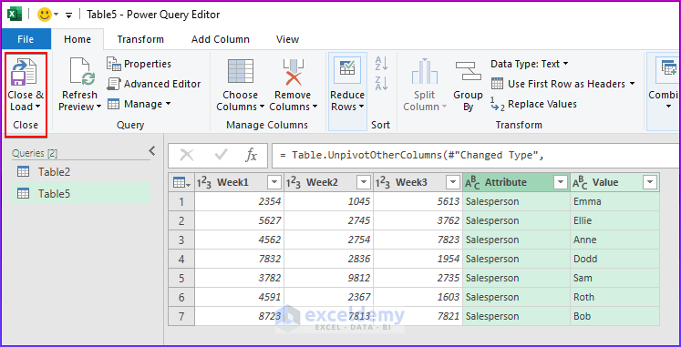
- The result will be a new worksheet containing the expected list.
Read More: How to Convert Range to Table in Excel
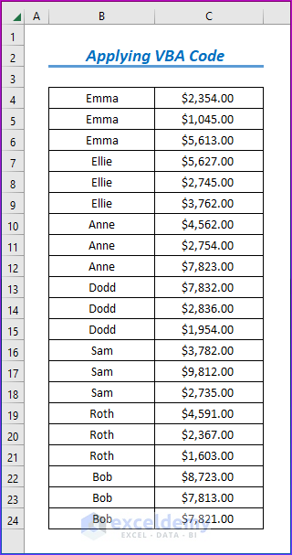
Method 3 – Applying VBA Code to Transform a Table into a List in Excel
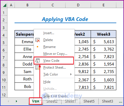
- Right-click on the sheet title where your data is located.
- Select View Code from the context menu.
- This will open the VBA window.
- Enter the VBA Code:
- Create a new subroutine called TransposeThis() (you can choose any name).
- Define the input and output ranges:
- TheRange : Set it to the data range you want to convert (e.g., Sheets(“VBA”) .Range(B5:B11)).
- TheRange_output : Set it to the location where you want the list output (e.g., Sheets(“sheet4”) .Range(“B2”)).
- Loop Through Rows:
- Use a For loop to iterate through each row in TheRange.
- For each row, determine the range of values to be transposed:
- range_values : Set it to the cells from the current row (excluding the first cell) up to the last non-empty cell in that row.
- Check Condition:
- If the number of cells in range_values less than 15,000 (you can adjust this threshold), proceed with the transposition.
- Assign Values:
- Inside the loop, assign the value from TheRange to TheRange_output.
- Offset TheRange-output by one column and assign the corresponding value from range_values.
- Move to Next Row:
- Offset TheRange_output by one row to prepare for the next row’s output.
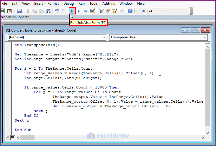
Sub TransposeThis()
Set TheRange = Sheets("VBA").Range("B5:B11")
Set TheRange_output = Sheets("sheet4").Range("B2")
For i = 1 To TheRange.Cells.Count
Set range_values = Range(TheRange.Cells(i).Offset(0, 1), TheRange.Cells(i).End(xlToRight))
If range_values.Cells.Count < 15000 Then
For j = 1 To range_values.Cells.Count
TheRange_output.Value = TheRange.Cells(i).Value
TheRange_output.Offset(0, 1).Value = range_values.Cells(j).Value
Set TheRange_output = TheRange_output.Offset(1, 0)
Next j
End If
Next i
End Sub- Press the Play icon (usually a green triangle) to execute the VBA code.
By following these steps, you’ll obtain your desired list in a new sheet.
Download Practice Book
You can download the practice workbook from here:
Further Readings
- Excel Table vs. Range: What Is the Difference?
- Navigating Excel Table
- How to Make Excel Tables Look Good
- Table Name in Excel: All You Need to Know
- How to Insert Floating Table in Excel
- How to Make a Comparison Table in Excel
- How to Create a Table Array in Excel
- How to Provide Table Reference in Another Sheet in Excel
<< Go Back to Excel Table | Learn Excel
Get FREE Advanced Excel Exercises with Solutions!

Hi, tried the first 2 methods, really useful thank you. Would it be possible to include an additional category on the left, eg the region of the salesperson?
Hello Jane, thanks for your feedback.
Yes, it’s possible, just add the column on the left and apply the commands as I applied.