Latest Posts From Md. Sourov Hossain Mithun

Sometimes, we need to protect our Excel sheets or workbooks containing important data or calculations for security issues. If you remember the password then ...

Toolbar in Excel: Knowledge Hub Types of Toolbars in MS Excel How to Show Toolbar in Excel How to Restore Toolbar in Excel How to Hide Toolbar in ...

Uses of MS Excel: Knowledge Hub How to Use Microsoft Excel for Beginners << Go Back to Learn Excel

A complex number is a combination of real numbers and imaginary numbers represented in x+iy format. Where x is the real part and y is the coefficient of the ...

Excel Combo Chart: Knowledge Hub How to Create a Combination Chart in Excel How to Combine Two Graphs in Excel How to Create Column and Line Chart ...

Here’s the sample dataset that we’ll use to demonstrate the examples. It represents some salespersons’ sales and dates in different regions. We'll ...

Method 1 - Use Only COUNTIF Function to Compare Two Columns in Excel Steps: Type the following formula in Cell E5- =COUNTIF($C$5:$C$11,D5) ...
![[Fixed!] IF Function Is Not Working in Excel (4 Solutions)](https://www.exceldemy.com/wp-content/uploads/2022/11/If-Function-Not-Working-in-Excel-11.png)
The sample dataset records person’s name and gender. Solution 1 - Remove Leading Space A leading space is the most common reason why a formula ...

The sample dataset contains students' marks in two subjects. We will fill with green or yellow to highlight marks greater than 80 or less than 50 respectively. ...

Here’s our sample dataset which contains 5 files in a folder named ExcelDemy. We'll copy the names to an Excel sheet. Method 1 - Using the Shortcut ...

In this article, we’ll demonstrate 3 easy methods to copy a table from Excel to Word. To illustrate our methods, we'll use the following dataset, a table that ...

This is the sample dataset. Method 1 - Using the Ampersand to Concatenate Email Addresses in Excel Steps: In C11, enter the following formula ...

Method 1 - Mark Indicator Only, and Comments and Notes on Hover Option Solution: Click the File tab beside the Home tab. Click on Options from ...

Slack time is a significant factor in project management. To finish a project on time, finding slack time is reasonably necessary. If you don't know what slack ...
Method 1 - Calculating Individual Person-Based Absenteeism Percentage Steps: Insert the following absenteeism formula into Cell F5- =E5/C5 ...
- 1
- 2
- 3
- …
- 14
- Next Page »
See Our Reviews at


Hello CJ, thanks for your feedback.
Just skip the percentage if it doesn’t get relevant, the formula and procedures are the same.
Hello JEMAIMAH OMAKEN, thanks for your feedback.
Visit our site to explore more articles that will work on Excel 2013. As 2013 is not so older version so you will find no major differences.
Hello Jane, thanks for your feedback.
Yes, it’s possible, just add the column on the left and apply the commands as I applied.
Hello ROY, thanks for your feedback. You have got a nice trick. I hope, it will help others.
But if the reverse order affects the other calculation of any user then maybe the alternative methods are more feasible.
Hello ANDY S, thanks for your feedback.
I hope the following codes will be helpful for your problem.
Sub Print_Button_for_DropDown()
Sheets(“Data”).Range(“$B$4:$D$11”).AutoFilter Field:=2, Criteria1:=Range(“F4”).Value
Sheets(“Data”).Select
Sheets(“Data”).PrintOut
End Sub
Here, I have made a drop-down list in Cell F4 for the locations. Keep this cell in that sheet where the print button is located, that means the active sheet. You can change the reference and range in the codes according to your dataset.
Hello JULIA MANDEVILLE,
We hope you are doing well. You got the exact mismatch between the code on the article and the code on the Excel file. That was very unfortunate and we really appreciate your feedback, thank you so much. We have fixed it on the article and Excel file.
Thanks and regards,
Md. Sourov Hossain Mithun
Team ExcelDemy
Hello MEGAN M,
Hope, you are doing well. Here’s the modified code below that will spell only whole numbers. Also, it will extract the whole number before spelling, if you insert decimal numbers.
Thanks and regards,
Md. Sourov Hossain Mithun
Team ExcelDemy.
Hello NYDA,
Thanks a lot for your suggestion. We worked on your suggestion but couldn’t find the exact reason for which your solution worked. We tried it on Excel 365, maybe it can be applicable to the earlier versions. So it would be great a favor for us if you would share your Excel version and the specific reason for the issue.
Thanks and regards,
Md. Sourov Hossain Mithun
Team ExcelDemy.
Hello PHIL REINIE,
Thanks for your feedback. The issue you introduced is really a valid issue that we never faced before. Thanks a lot for sharing it with us. We have added this solution in our article, we hope it will help other users.
Thanks and regards,
Md. Sourov Hossain Mithun
ExcelDemy
Hello MISTI,
Thanks for your feedback. I hope you will be glad to know that, we have updated our methods according to related examples. Now it will help you to understand the specific use of every method.
Hello WILL,
Thanks for your feedback. There are some reasons that are why you may have faced the problem. You can solve it by following the steps:
1. Maybe your Fill Handle tool is deactivated. To activate it, Click File > Options > Advanced > Enable fill handle and cell drag and drop.
2. The AGGREGATE function can work only for vertical ranges, not for horizontal ranges. So always apply it for vertical ranges and then the Fill Handle should work.
3. The AGGREGATE function is available since 2010, so if you are using an older version of Excel then it won’t work.
If the above solutions fail to rescue you then your issue is quite particular and that is difficult to find out without the file. So if you share your file with us then we hope, we could provide you with the exact solution.
*Sharing Email Address: [email protected]
Hello EYAD,
Thanks for your feedback. It’s possible to combine 3 columns using the 2nd method after a little bit modification of the formula.
I added more 4 products in column D and then applied this formula in Cell E5:
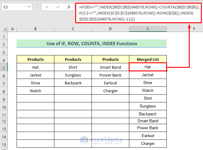
=IF(B5<>"",INDEX($B$5:$B$1048576,ROW()-COUNTA($B$5:$B$8)),IF(C1<>"",INDEX($C$5:$C$1048576,ROW()-ROW($E$8)),INDEX($D$5:$D$1048576,ROW()-11)))*INDEX($D$5:$D$1048576,ROW()-11)
Here, 11 is used based on the length of the second column.
Hello ROXY,
Thanks for your feedback. The above three issues are all the most common and possible issues that we have recognized till now. Would you please check whether your worksheet is protected or not? If not then maybe your problem is quite particular and that’s quite difficult to find without the file. So if you would share your file with us then hope, we could find out the reason and give a proper solution.
*Sharing email address: [email protected]
Hello DILEKA,
Thanks for your feedback. There are some possible reasons for why the sort command may not work:
1. Remaining blank rows, cells, or blank columns in the selected range.
2. Presence of Leading Space.
3. Mixed Data Type in the Same Column.
4. Selecting multiple worksheets before sorting.
To know in detail, please follow this article regarding on this issue:
https://www.exceldemy.com/sort-and-filter-in-excel-not-working/#Sort_and_Filter_are_Greyed_out_in_Excel
We hope the above solutions will rescue you. If not, then your problem is quite particular. In that case, if you share your worksheet with us then hope, we will be able to find out the issue and give a proper solution.
Hello DANIEL,
Yes, it’s possible to do that using the COUNTA function based on the first column. For that, use the following formula-
=IF(B5<>"",INDEX($B$5:$B$1048576,ROW()-COUNTA($B$5:$B$8)),INDEX($C$5:$C$1048576,ROW()-COUNTA($B$5:$B$8)-4))➥
ROW()-COUNTA($B$5:$B$8)-4Here, 4 is subtracted based on the length of the first column to return 1 as the output of this portion. So for your own dataset, modify the value according to the length of your first column.
Hello TAB,
Thanks for your feedback. You can easily do that by using a simple formula.
Follow the steps:
1. Select the range of dates.
2. Click on the Conditional Formatting command from the Home tab.
3. Then select New Rule.
4. Select “Use a formula to determine which cells to format”.
5. After that, insert the formula in the “Format values where this formula is true box”-
=AND(D1<=TODAY(),F1<>"Complete")6. Choose the Red fill color from the Format command.
7. Finally, hit the OK button.
*To gray out the dates with complete status, use the following rule and Gray fill color:
=AND(D1<=TODAY(),F1="Complete")Hello JULIE, thanks for your feedback. Use the below code to fix that-
Sub Worksheet_SelectionChange(ByVal Target As Range)
Static xRow
Cells.Interior.ColorIndex = 0
If xRow “” Then
With Rows(xRow).Interior
.ColorIndex = xlNone
End With
End If
Active_Row = Selection.Row
xRow = Active_Row
With Rows(Active_Row).Interior
.ColorIndex = 7
.Pattern = xlSolid
End With
End Sub
*Or you can use an alternative way with the previous code, after opening the file, click on any cell on the previously highlighted row, and then only the active row will be highlighted.
Hello JK,
Thanks for your feedback. Your problem is quite rare and unique. So it’s difficult to detect this type of problem without the user’s Excel file. If you would share your file with us, then hopefully we could detect the issue and could give you the exact solution. But temporarily we are suggesting you use the SUM function within the TRIM function, we are showing you a sample formula:
=TRIM(SUM(C5:C9))
The TRIM function will remove all extra spaces. I hope, it will help you.
Hello HERMAN,
Thanks for your feedback. You can follow the articles given below to create a payroll format based on 15 days. The steps and format will be pretty same, hope it will help you.
https://www.exceldemy.com/daily-wages-sheet-format-in-excel/#Step_1_Calculate_Total_Daily_Working_Time_in_Daily_Wages_Sheet_Format_in_Excel
https://www.exceldemy.com/calculate-hours-and-minutes-for-payroll-in-excel/
Hello KATHY,
Thanks for your feedback. Would you please check whether your worksheet is protected or not? If not then your problem is quite specific. So if you would share your file with us then hope, we could find out the reason and provide a solution.
Hi MICHAEL,
Thanks for your feedback.
To count the number of items associated with each title (according to to catalog id), use this formula: =COUNTIF($B$2:$B$27,B2)
And to sum the total number of uses of each item associated with that same title, use this formula: =SUMIF($B$2:$B$27,B2,$D$2:$D$27)
Hello Mat, thanks for your feedback. The problem you mentioned will need a complex formula. You will have to apply a formula like this:
=IF(SUM(–(MAX(AC2:AC12)=AC2:AC12))=1,INDEX(T2:AC12,MATCH(MAX(AC2:AC12),AC2:AC12,0),1)).
Hello HOPE, thanks for your feedback. To do that, place Private Sub Workbook_open() in a new module and then call the previous Sub within it. I hope, it will work.
Hello Mahedi, thanks for your feedback. When you download the file then there’s no connection between your downloaded file and our uploaded file. So, no worries, your file won’t lose.
Hello TONIA.
Thanks for your feedback. Autofit doesn’t work in a protected sheet, so please check it. If it remains unprotected then your problem is a quite particular type. So if you would share your workbook with us, we hope to find out the problem and give you a possible solution.
Hello, HPOTTER.
Thanks for your feedback. We think your problem is very specific which is difficult to identify without the file. So, if you would share your Excel file with us then we could find out the issue and hope, we could give you a solution.
You are welcome 🙂 Glad to know that it helped you.