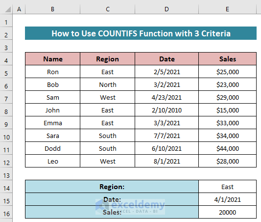
How to Use COUNTIFS Function with 3 Criteria in Excel

Here’s the sample dataset that we’ll use to demonstrate the examples. It represents some salespersons’ sales and dates in different regions. We’ll count the cells which meet the three criteria: Region=East, Date<=4/1/2021, and Sales>=20000.

Example 1 – Insert the Criteria Directly in the COUNTIFS Function

Steps:

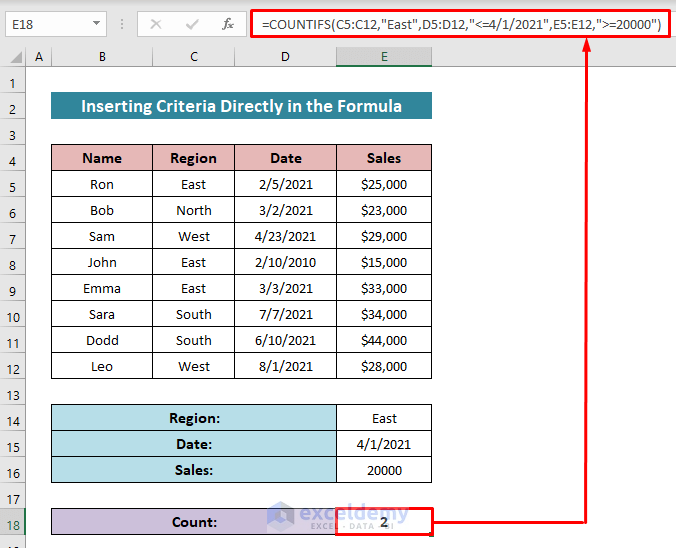
Activate Cell E18.
Use the following formula in it-

=COUNTIFS(C5:C12,"East",D5:D12,"<=4/1/2021",E5:E12,">=20000")

Hit the Enter button to get the number of cells that meet all criteria.

Example 2 – Apply Criteria Using the Ampersand and Cell References in the COUNTIFS Function

Steps:

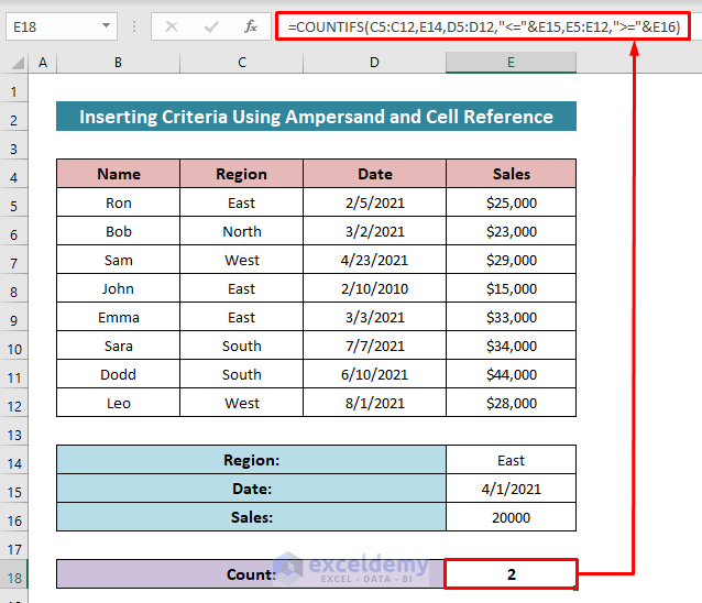
Cells E14 through E16 contain the values that need to be checked.
In Cell E18, insert the following formula-

=COUNTIFS(C5:C12,E14,D5:D12,"<="&E15,E5:E12,">="&E16)

COUNTIFS implicitly converts cell references to their values. The ampersand operator converts these values to text and joins them with the operators that will create a logical check.

Press the Enter button to get the result.

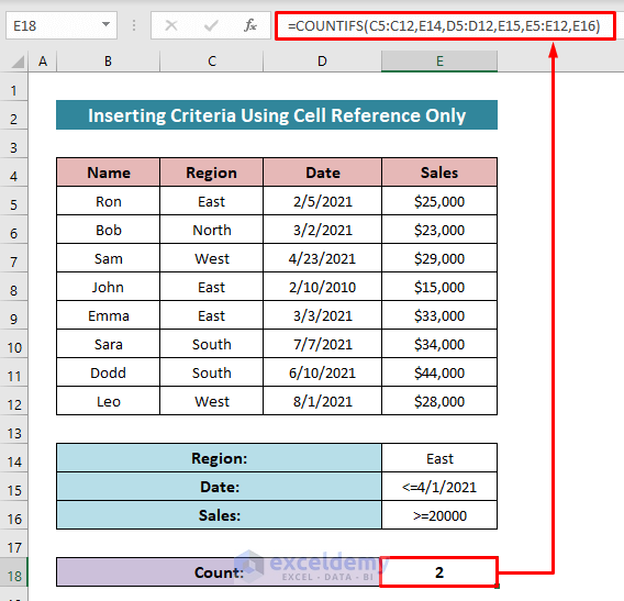
Example 3 – Perform Criteria Using the Cell Reference Only

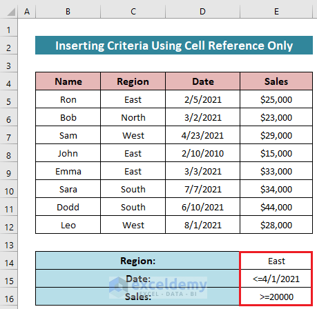
We modified the criteria list in the dataset. We inserted the ‘less than or equal to’ sign and the ‘greater than or equal to’ signs in the dataset.

Steps:

Insert the following formula in Cell E18:

=COUNTIFS(C5:C12,E14,D5:D12,E15,E5:E12,E16)

Hit the Enter button.

Remarks

127 pairs of criteria ranges and criteria can be inserted.
If any reference for the criteria remains empty (i.e, the formula has two commas side by side), the COUNTIFS function will consider it as “equals zero”.

Download the Practice Workbook

3 Criteria in COUNTIFS Function.xlsx