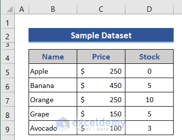
The COUNTIFS function is a more advanced version of the COUNTIF function in Excel. Whereas the COUNTIF function counts if one criterion in a single range is satisfied, the COUNTIFS can count if multiple criteria in multiple ranges are satisfied. In this article, we will discuss nine advanced uses of the COUNTIFS function in Excel, using the following dataset as the basis to illustrate our methods.
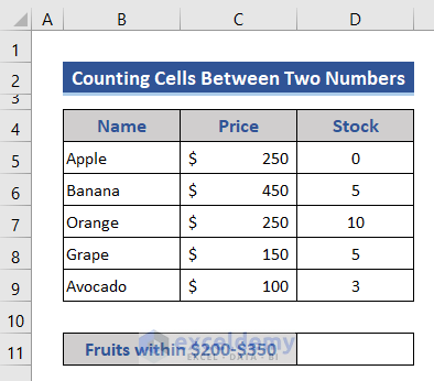
Example 1 – Counting Cells Between Two Numbers
In the first example, we’ll count the number of cells between two specified numeric values in Excel using the COUNTIFS function.
Steps:
- Add a row to the dataset that contains two cells, B11:D11. Name the left appropriately, and keep the right cell blank for now.
- Enter the following formula in cell D11:
=COUNTIFS(C5:C9,"<350",C5:C9,">200")
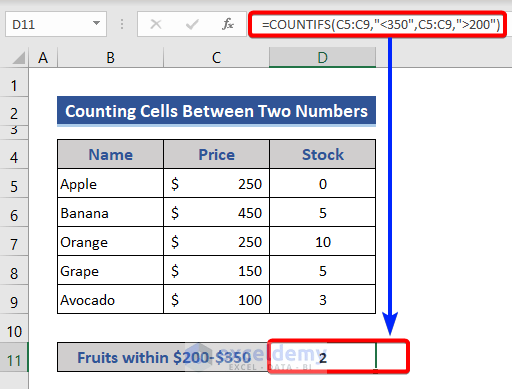
Here, we applied two conditions in the same column to count the number of rows where the price is (i) less than $350, and (ii) greater than $200.
Note: Always enter greater or less than criteria inside double quotes “”, for example. “>200”, or “>=300”.
Example 2 – Combining COUNTIFS with the EDATE Function to Count Values That Meet a Date Criteria
Here, we’ll insert date values in the COUNTIFS function using cell references, and use the EDATE function for previous or future dates.
We modified the dataset for this example, adding the expiry date of the products.
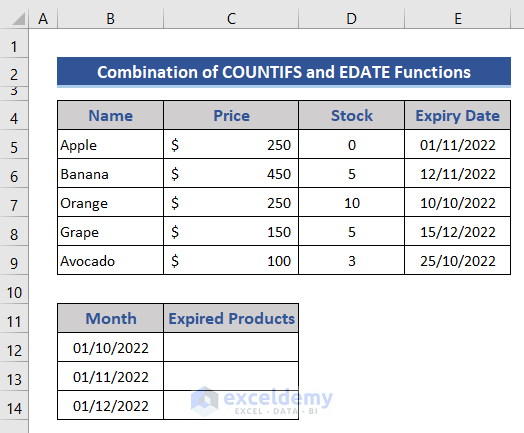
In the result section, we insert 3 dates. We want to know the number of products with an expiry date 1 month later than these dates. We’d like to show the month names rather than the dates, but since the EDATE function does not recognize month names, we’ll have to do this by changing their format.
Steps:
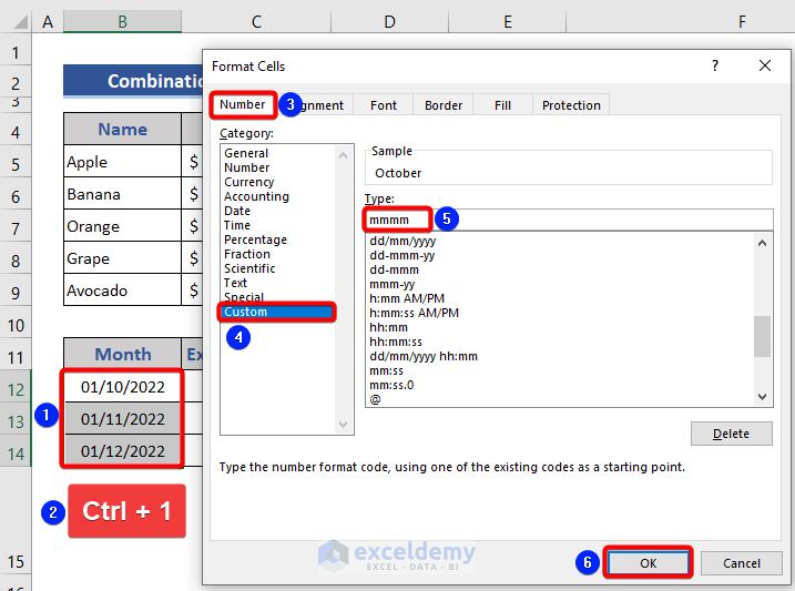
- Select the range B12:B14.
- Press the keyboard shortcut Ctrl+1 to open Format Cells.
- Choose the Custom option from the Number tab.
- Input the format in the Type box like in the picture below and click OK.
The result is as follows:
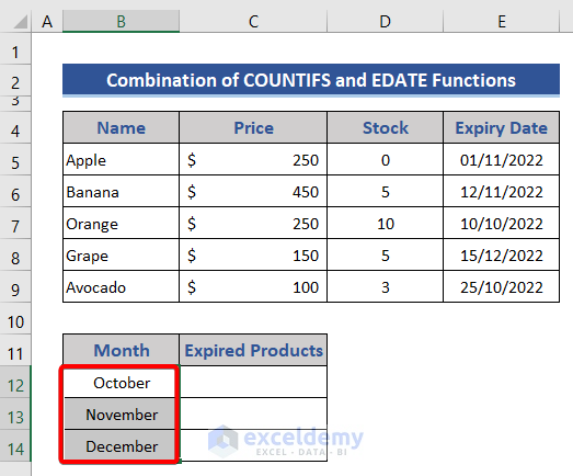
The dates are now shown in terms of their corresponding month’s name.
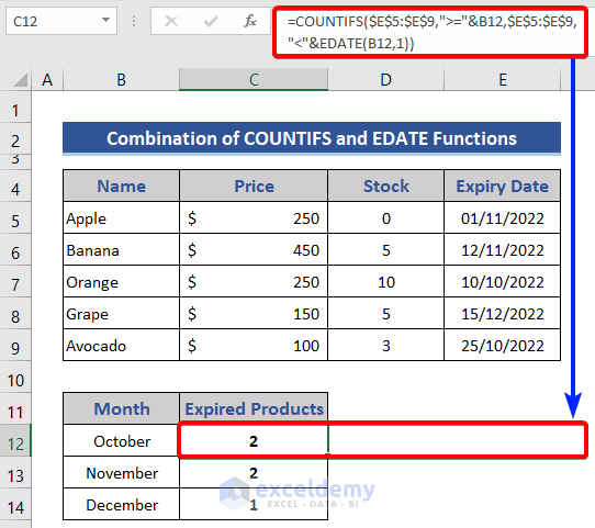
- Enter the following formula in cell C12:
=COUNTIFS($E$5:$E$9,">="&B12,$E$5:$E$9,"<"&EDATE(B12,1))
- Press Enter and drag the Fill Handle icon down to copy the formula for the other months below.
Note:
- We can alternatively use the DATE function to insert date values in the formula:
=COUNTIFS($E$5:$E$9,">="&DATE(2022,10,1),$E$5:$E$9,"<"&EDATE(DATE(2022,10,1),1))
- We can also insert hardcoded dates:
=COUNTIFS($E$5:$E$9,">="&"1/10/2022",$E$5:$E$9,"<"&EDATE("1/10/2022",1))
Read More: How to Use COUNTIFS with Date Range in Excel
Example 3 – Using the COUNTIFS Function with Multiple OR Criteria in Different Columns
Now we’ll use the COUNTIFS function to perform OR operations based on different columns.
Steps:
- Set a condition, like in the image below.
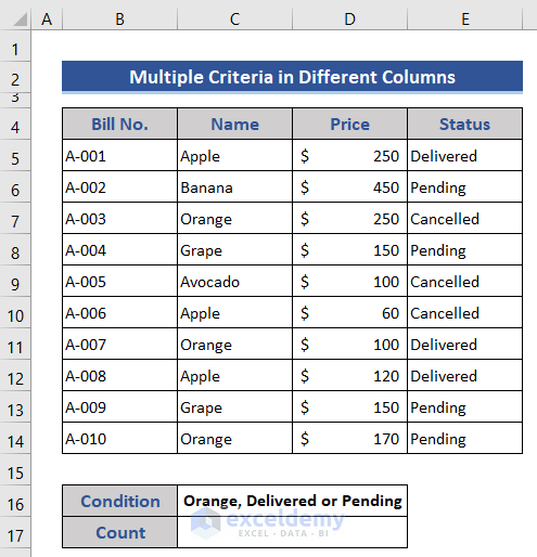
We’ll find the number of cells containing Orange, that either have a status of Delivered or Pending.
- Enter the formula below in cell C17:
=COUNTIFS($C$5:$C$14, "Orange", $E$5:$E$14,"Delivered") + COUNTIFS($C$5:$C$14, "Orange",$E$5:$E$14,"Pending")
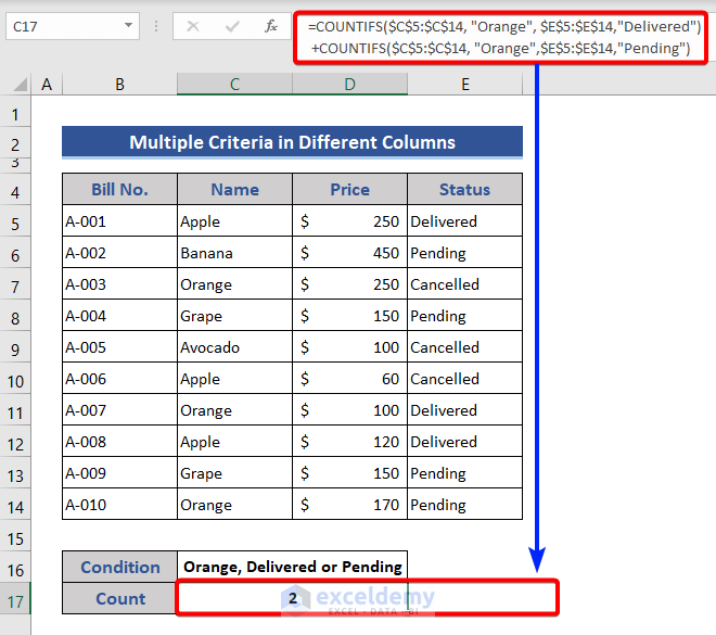
Here, we combine two COUNTIFS functions and return their OR result. The first part of this formula returns the number of orange bills that are Delivered, and the 2nd part returns the number of orange bills that are Pending.
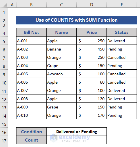
Example 4 – Using the COUNTIFS Function to Sum with OR Logic
We will combine the SUM and COUNTIFS functions here, and apply the conditions in an array form in the formula.
Steps:
- Set a condition of which products have a Status of Delivered or Pending.
- Insert the following formula in cell C17:
=SUM(COUNTIFS($E$5:$E$14,{"Delivered","Pending"}))
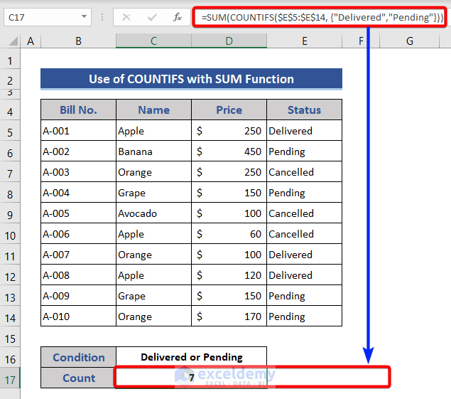
The result is the sum of delivered and pending products.
Example 5 – Advanced Use of the COUNTIFS Function with Wildcards
Now we will use a wildcard with the COUNTIFS function.
Steps:
We set a condition here of which cells contain both Bill No. and Price. We’ll use the wildcard for Bill No. and “not equal to” for the Price.
- Enter the following formula in cell C17:
=COUNTIFS($B$5:$B$14,"*",$D$5:$D$14,"<>"&"")
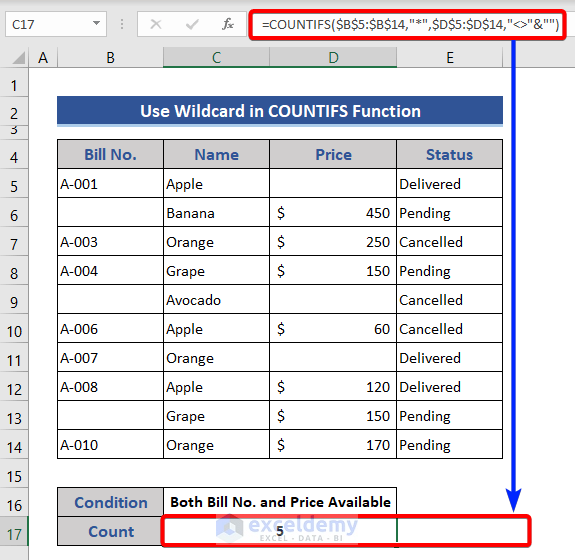
The result above is obtained due to the wildcard symbol.
Example 6 – Using the COUNTIFS Based on the Current Day
Next, we will combine the TODAY function with the COUNTIFS function. We’ll find the number of products that are packaged before the present day, and those that expire after the present day.
Steps:
- Input the following formula in cell C12:
=COUNTIFS(E5:E9, "<"&TODAY(),F5:F9, ">"&TODAY())
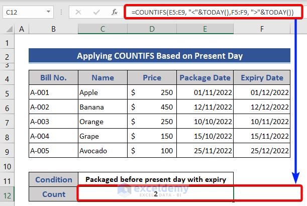
The correct result is returned.
Example 7 – Inserting Numeric and Text Criteria Within the COUNTIFS Function
We can insert both numeric and text conditions simultaneously in the COUNTIFS function.
Steps:
- Enter the following formula in cell C17:
=COUNTIFS($C$5:$C$14, "Orange", $D$5:$D$14,"<=200")
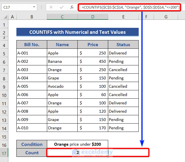
The result above is returned after inserting both numeric and text references in the function.
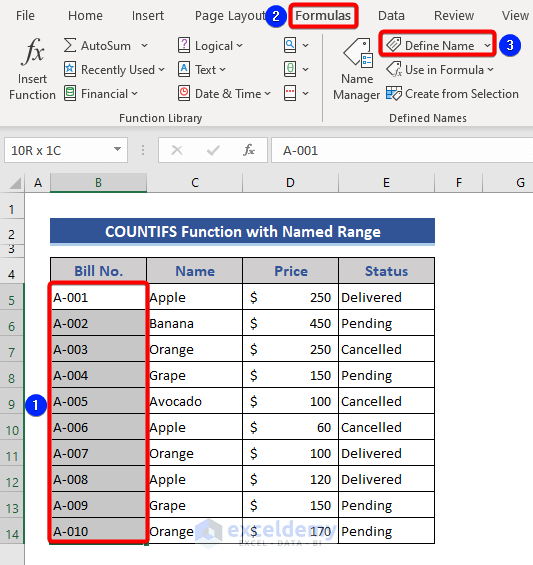
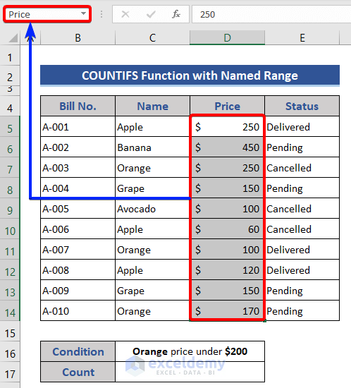
Example 8 – Using COUNTIFS with a Named Range
Steps:
First, let’s name a range:
- Select the data range of the Bill No. column.
- Go to the Define Name section of the Formulas tab.
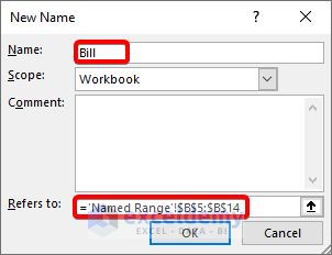
The New Name window appears.
- Enter a name in the Name Box.
The selected range can be seen in the Refers to section.
We can also define names in a simple way:
- Just select the data range of the Name column and put a name in the Name Box in the upper-left side of the sheet.
- Press Enter.
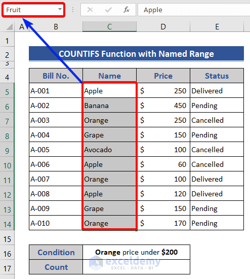
- Similarly, set the name of the data range for the Price column.
- Insert the following formula in cell C17:
=COUNTIFS(Fruit,"Orange",Price,"<=200")
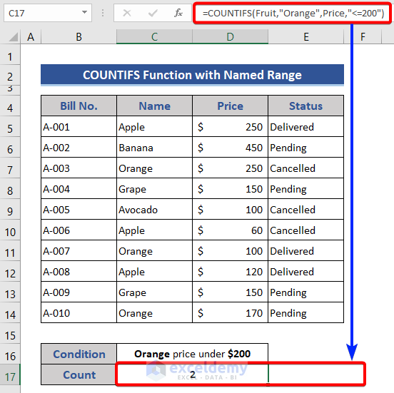
In this formula, we used the named range as the reference, greatly simplifying the syntax.
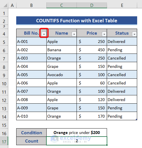
Example 9 – Using the COUNTIFS Function in an Excel Table
The table is a very useful feature of Excel. Let’s use one to create a formula.
Steps:
Let’s first create a table:
- Select the whole dataset.
- Press Ctrl + T to create a table.
The selected range is displayed in the Create Table window.
- Mark the My table has headers option.
- Click OK.
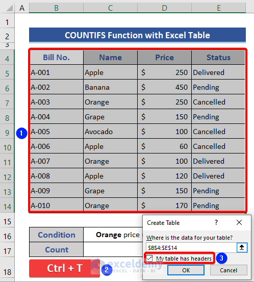
The table has been formed successfully.
- Enter the following formula in cell C17:
=COUNTIFS(Table1[Name],"Orange",Table1[Price],"<=200")
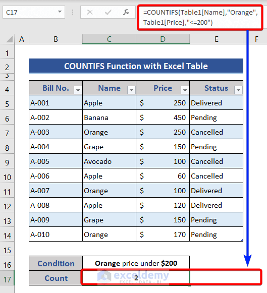
The same result is returned using the table as reference instead of cell references or named ranges.
Download Practice Workbook
Related Articles
- How to Use COUNTIFS for Cells Not Equal to Multiple Text in Excel
- How to Use COUNTIFS Function with 3 Criteria in Excel
<< Go Back to Excel COUNTIFS Function | Excel Functions | Learn Excel
Get FREE Advanced Excel Exercises with Solutions!
