Dataset Overview
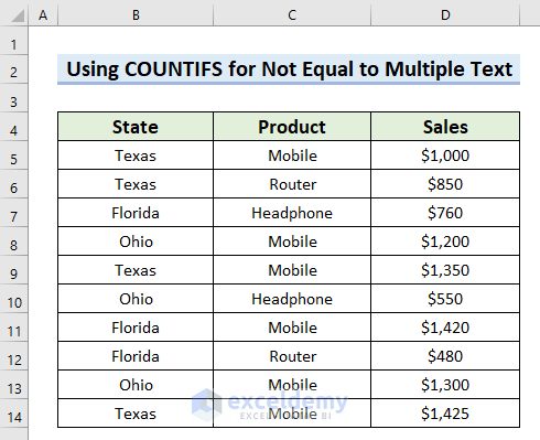
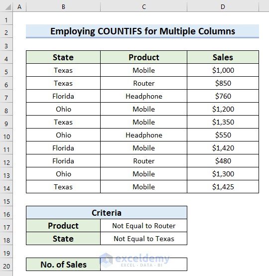
We’ll use the following dataset to explain these methods. It contains 3 columns, State, Product, and Sales.
Method 1 – COUNTIFS for Cells Not Equal to Multiple Text (Single Column)
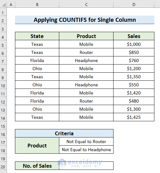
- Select the cell where you want to calculate the No. of sales (Cell C20).
- Enter the following formula in Cell C20:
=COUNTIFS(C5:C14,"<>Router",C5:C14,"<>Headphone")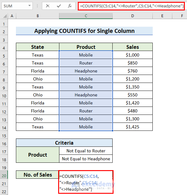
- Press Enter to get the result. The formula will return the number of cells that meet both criteria.
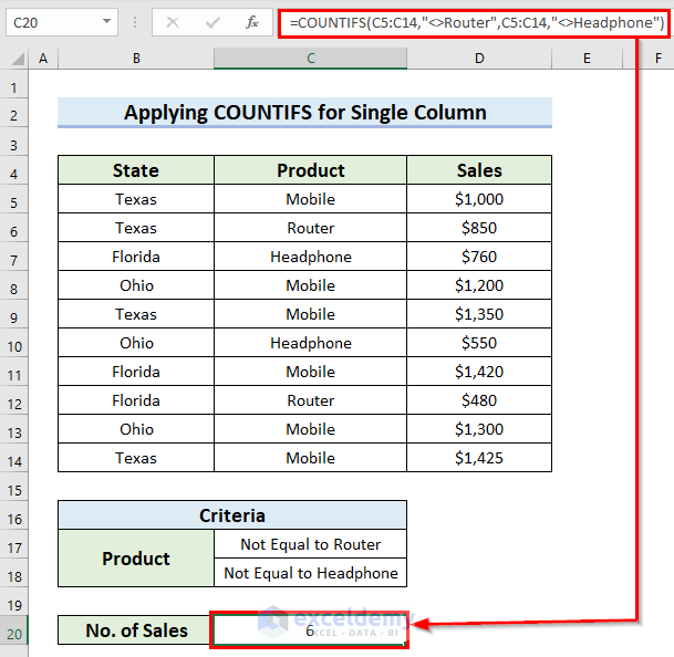
This formula counts the cells in the range C5:C14 where the product is not equal to Router and not equal to Headphone.
Method 2 – COUNTIFS for Cells Not Equal to Text (Multiple Columns)
- Select the cell where you want to calculate the number of sales.
- Enter the following formula in that selected cell:
=COUNTIFS(C5:C14,"<>Router",B5:B14,"<>Texas")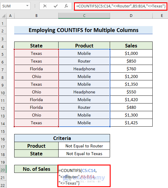
- Press Enter to get the result. The formula will return the number of cells that match both criteria.
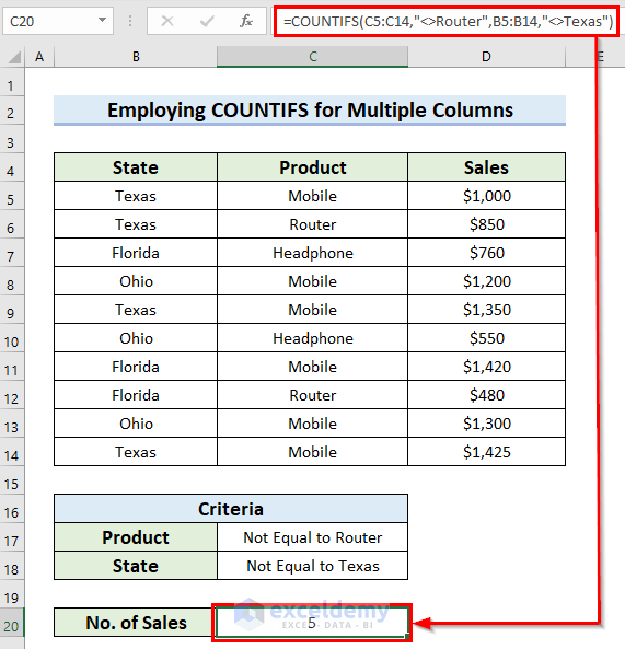
This formula counts the cells where the product is not equal to Router (in column C) and the state is not equal to Texas (in column B).
Alternative Solution to Count Cells If Not Equal to Multiple Text in Excel
In this section, we will use an alternative solution for counting the number of cells in this type of situation.
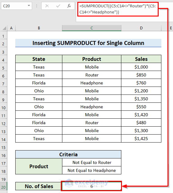
Alternative Method 1 – Using SUMPRODUCT
- Select the cell where you want to count the No. of Sales.
- Enter the following formula:
=SUMPRODUCT((C5:C14<>"Router")*(C5:C14<>"Headphone"))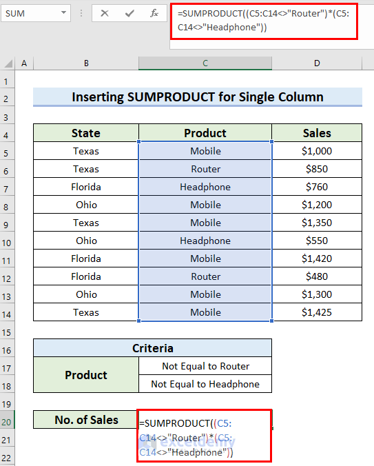
- Press Enter and you will get the No. of Sales.
- If you are using an older version of Microsoft Excel (prior to Excel 2019), press Ctrl + Shift + Enter after entering the formula.
How Does the Formula Work?
- This formula multiplies two arrays: one for cells not equal to “Router” and another for cells not equal to “Headphone.”
- It then sums up the results.
Alternative Method 2 – Count Cells for Criteria from Multiple Columns
- Select the cell where you want to calculate the No. of Sales Cell C20).
- Enter the following formula:
=SUMPRODUCT((B5:B14<>"Texas")*(C5:C14<>"Router"))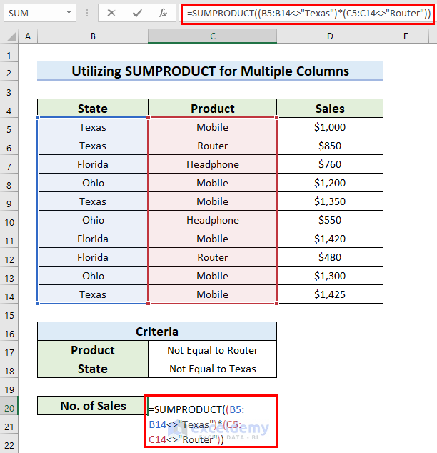
- Press Enter to get the result.
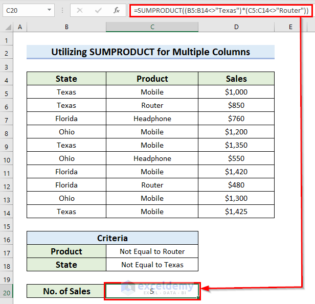
How Does the Formula Work?
- This formula multiplies the arrays for states not equal to “Texas” (in column B) and products not equal to “Router” (in column C).
Read More: Advanced Use of COUNTIFS Function in Excel
Things to Remember
- If you are using an older version of Microsoft Excel (prior to Excel 2019), press Ctrl + Shift + Enter for the array formula.
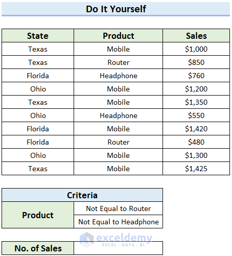
Practice Section
A practice sheet has been provided for you to practice how to use COUNTIFS for cells if not equal to multiple text in Excel.
Download Practice Workbook
You can download the practice workbook from here:
Related Articles
<< Go Back to Excel COUNTIFS Function | Excel Functions | Learn Excel
Get FREE Advanced Excel Exercises with Solutions!
