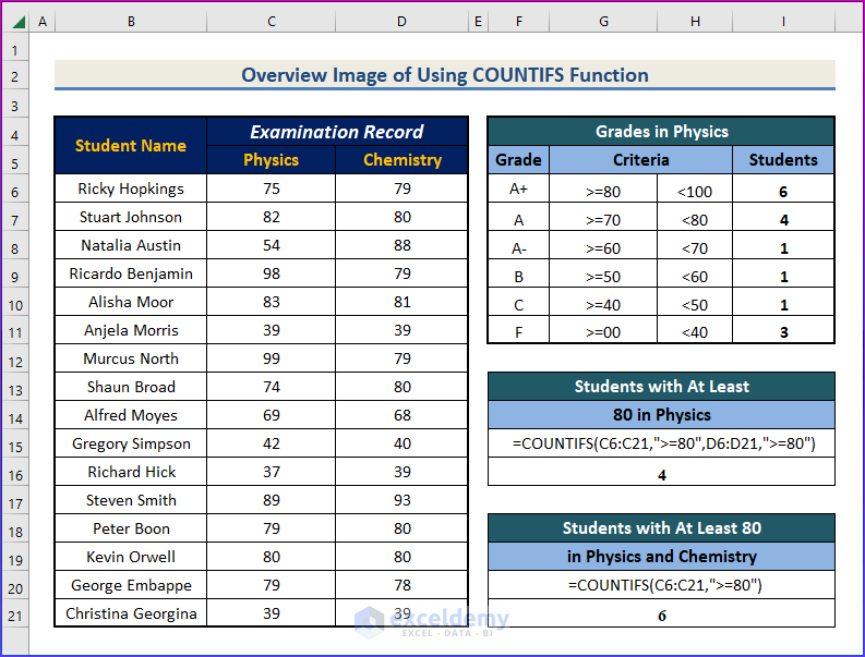
Here is an overview of using the COUNTIFS function.
Introduction to the Excel COUNTIFS Function
Objectives:
- Counts the number of cells in one or more given arrays that meet one or more specific criteria.
Syntax:
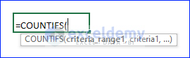
=COUNTIFS(criteria_range1,criteria1,...)Arguments Explanation:
| Argument | Required or Optional | Value |
|---|---|---|
| criteria_range1 | Required | The first array. |
| criteria1 | Required | Criteria applied to the first array. |
| criteria_range2 | Optional | The second array. |
| criteria2 | Optional | Criteria applied to the second array. |
| … | … | … |
Return Value:
- Returns the total number of values in the array that meet the criteria.
Version:
- The function is available from Microsoft Excel 2010.
Notes
- Only one criterion and one range of values where the criterion will be applied (criteria_range) is compulsory. But you can use as many criteria and as many ranges as you wish.
- The criteria can be a single value or an array of values. If the criteria include an array, the formula will turn into an Array Formula.
- The criteria and the criteria_range must come in pairs. That means if you input criteria_range 3, you must input criteria3.
- The lengths of all the criteria_ranges must be equal. Otherwise, Excel will raise #VALUE! Error.
- While counting, Excel will count only those values that satisfy all the criteria.
COUNTIFS Function in Excel: 4 Examples
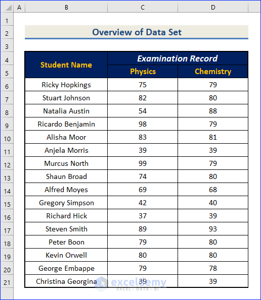
Suppose we have a sample dataset of students and their scores in two subjects.
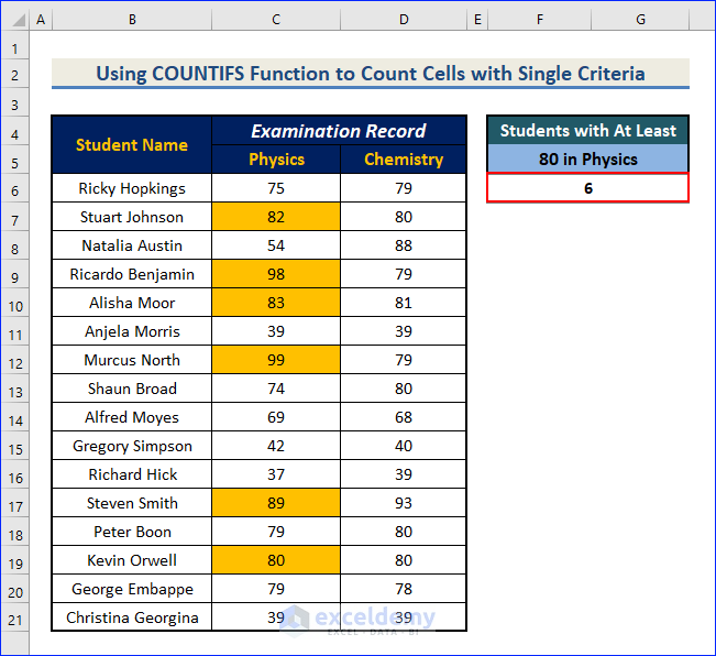
Example 1 – Using the COUNTIFS Function to Count Cells for a Single Criterion
Steps:
- We want to count how many students got at least an 80 in Physics.
- Use the following formula in the result cell.
=COUNTIFS(C6:C21,">=80")- Hit Enter.
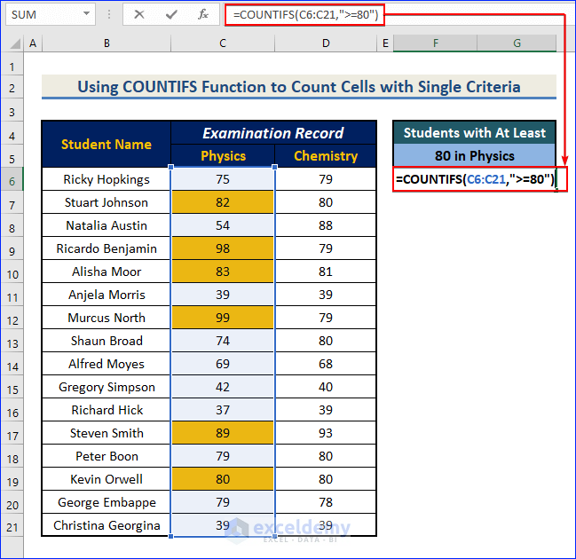
- You can see that there are 6 students who got at least 80 in Physics.
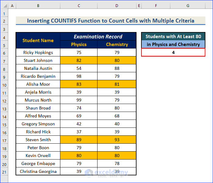
Example 2 – Inserting the COUNTIFS Function to Count Cells with Multiple Criteria
Steps:
- We will count how many students got at least 80 in both Physics and Chemistry.
- Use the following formula in the result cell.
=COUNTIFS(C6:C21,">=80",D6:D21,">=80")- Press Enter.
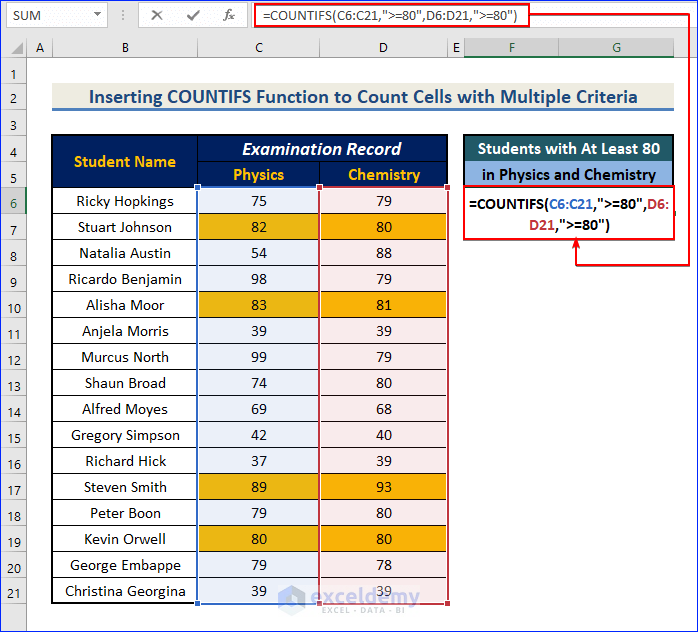
- Four students got at least 80 in both subjects.
Read More: How to Use COUNTIFS Function with 3 Criteria in Excel
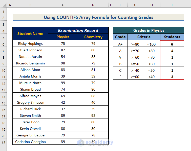
Example 3 – Using the COUNTIFS Array Formula for Grades in Excel
Steps:
- Let’s count the number of students with each grade in Physics.
- We put the criteria for each grade in a table to the right.
- Select all the cells in the empty result column, enter this formula in the first cell, and then press Ctrl + Shift + Enter.
=COUNTIFS(C6:C21,G6:G11,C6:C21,H6:H11)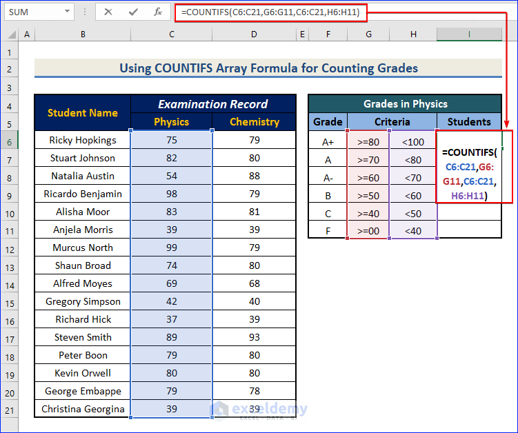
Formula Breakdown
- If we break down the array formula COUNTIFS(C6:C21,G6:G11,C6:C21,H6:H11), we will find six single formulas.
- COUNTIFS(C6:C21,G6,C6:C21,H6)
- COUNTIFS(C6:C21,G7,C6:C21,H7)
- COUNTIFS(C6:C21,G8,C6:C21,H8)
- COUNTIFS(C6:C21,G9,C6:C21,H9)
- COUNTIFS(C6:C21,G10,C6:C21,H10)
- COUNTIFS(C6:C21,G11,C6:C21,H11)
- COUNTIFS(C6:C21,G6,C6:C21,H6) returns the total number of cells in the range C6 to C21 that maintain the criteria G6 and H6.
- We have a breakdown of Physics grades.
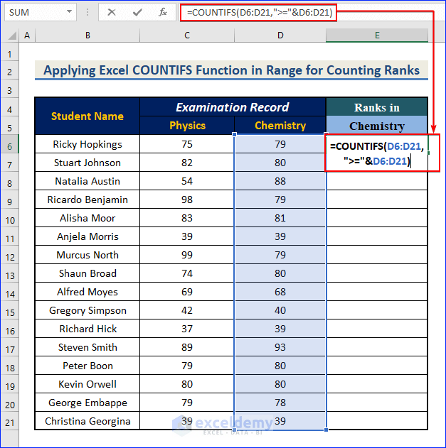
Example 4 – Applying the Excel COUNTIFS Function in a Range for Counting Ranks
Steps:
- We will get the rank of each student according to their marks in Chemistry.
- Select a new column and enter this formula in the first cell of the column.
=COUNTIFS(D6:D21,">="&D6:D21)- Press Ctrl + Shift + Enter.
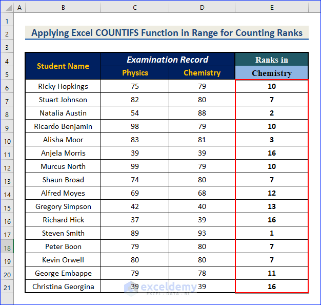
Formula Breakdown
- If we break down the array formula COUNTIFS(D5:D20,”>=”&D5:D20), we will find 16 different formulas.
- COUNTIFS(D6:D21,”>=”&D6)
- COUNTIFS(D6:D21,”>=”&D7)
- COUNTIFS(D6:D21,”>=”&D8)
- …
- …
- COUNTIFS(D6:D21,”>=”&D20)
- COUNTIFS(D6:D21,”>=”&D6) counts how many values in the array D6 to D21 have values greater than or equal to the value in D6. This is actually the rank of D6.
- Here are the results.
Things to Remember
- When the criterion denotes equal to some value or cell reference, just put the value or the cell reference in place of the criteria.
- When the criterion denotes greater than or less than some value, enclose the criteria within an apostrophe (“ ”).
- When the criterion denotes greater than or less than some cell reference, enclose only the greater than or the less than symbol within an apostrophe (“”) and then join the cell reference by an ampersand (&) symbol.
Common Errors with COUNTIFS Function
- #VALUE shows when the lengths of all the arrays are not the same.
Download the Practice Workbook
Excel COUNTIFS Function: Knowledge Hub
- How to Use COUNTIFS with Date Range in Excel
- Advanced Use of COUNTIFS Function in Excel
- How to Use COUNTIFS for Cells Not Equal to Multiple Text in Excel
- Excel COUNTIFS Not Working [Fixes]
<< Go Back to Excel Functions | Learn Excel
Get FREE Advanced Excel Exercises with Solutions!

It was so amazing that you are providing practice sheet for the excel
Hello Manjeet,
Glad to hear that our practice is sheet is helpful to you. We provide Excel practice sheet so that users can practice all the explained methods to develop Excel skills.
thanks for your appreciation and feedback.
Regards
ExcelDemy