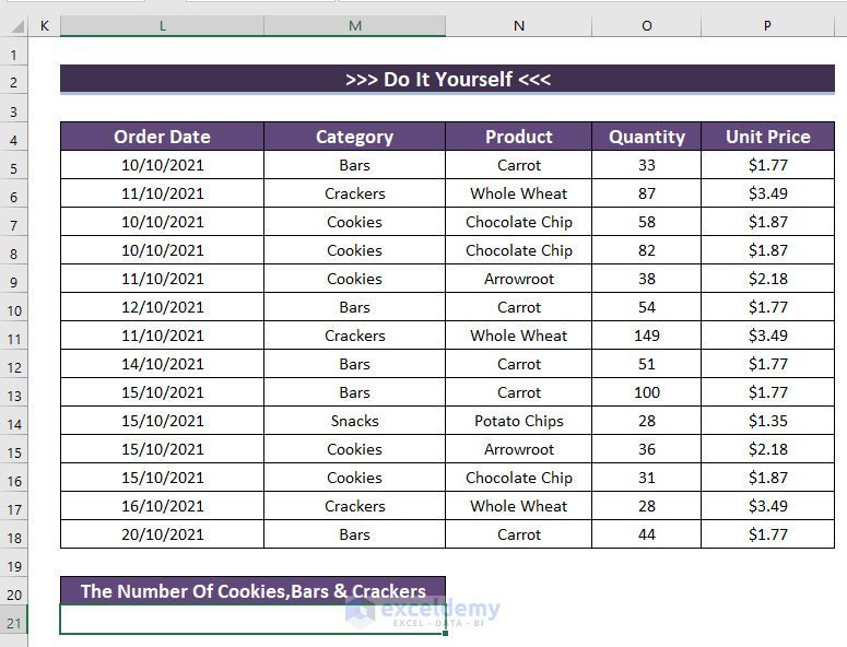
The sample dataset has the Order Date, Category, Product, Quantity, and Unit Price columns. We’ll use COUNTIFS with criteria in it.
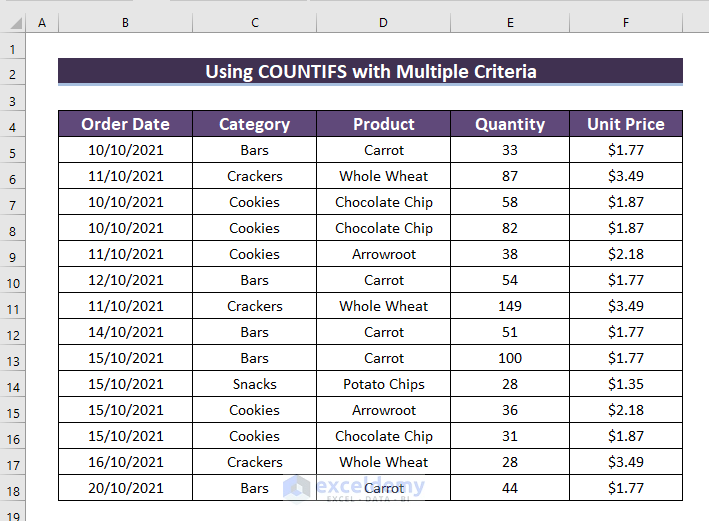
Example 1 – Applying the COUNTIFS Function with a Constant Array
We want to count the Cookies, Bars, and Crackers sales.
Steps:
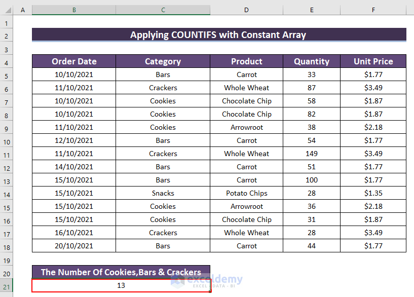
- Use the following formula in the merged cell B21:C21.
=SUM(COUNTIFS($C$5:$C$18,{"Cookies","Bars","Crackers"}))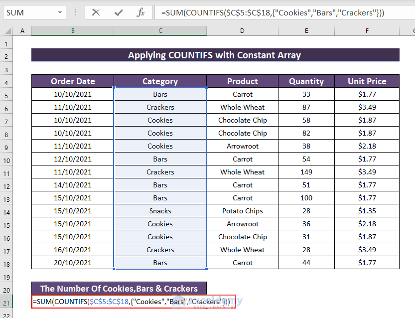
- Press Enter.
Example 2 – Using the COUNTIFS Function with Multiple Criteria for Different Values and Dates
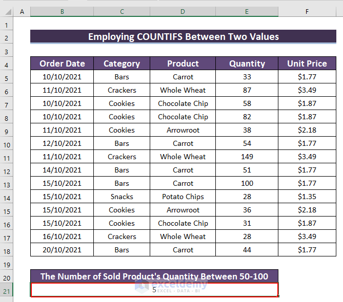
Case 2.1 – Between Two Values
We want count the number of products where the sold Quantity exceeds 50 but is below 100.
Steps:
- Use the following formula in the merged cells B21:E21.
=COUNTIFS($E$5:$E$18,">50", $E$5:$E$18,"<100")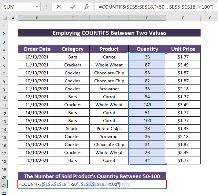
- Hit Enter.
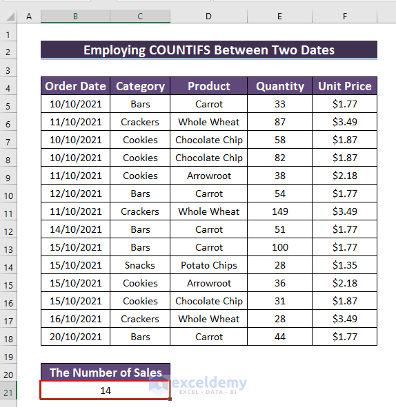
Case 2.2 – Between Two Dates
We’ll count the sales between 11/10/2021 to 15/10/2021.
Steps:
- Use the following formula in the merged cells B21:C21.
=COUNTIFS($B$5:$B$18,">="&DATE(2021,10,10),$B$5:$B$18,"<="&DATE(2021,10,20))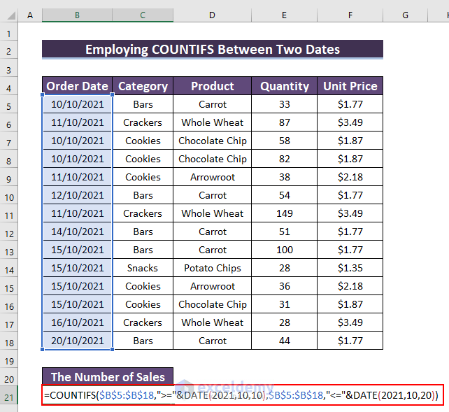
- Hit Enter.
Read More: How to Use COUNTIFS with Date Range and Text in Excel
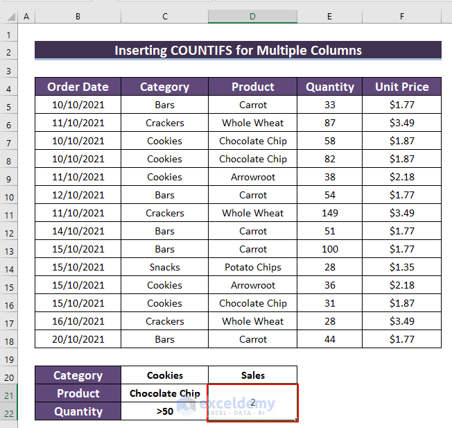
Example 3 – Inserting the COUNTIFS Function with Multiple Criteria in Multiple Columns
We’ll count the sales of products (Chocolate Chip) based on category (Cookies) and a specific quantity (>50).
Steps:
- List the criteria in C20, C21, and C22.
- Use the following formula in the merged cells D21:D22.
=COUNTIFS($C$5:$C$18,C20,D5:D18,C21,$E$5:$E$18,C22)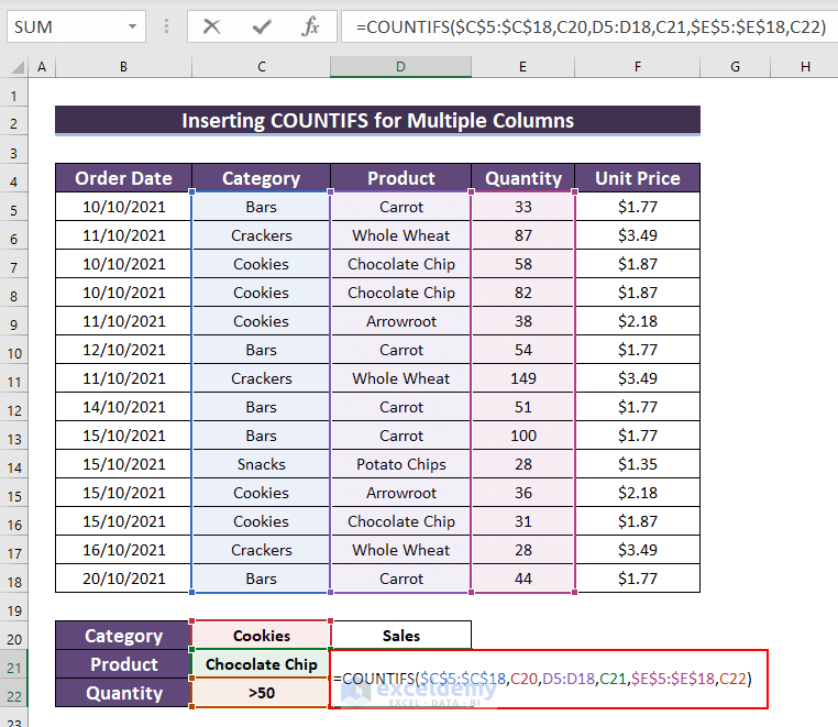
- Hit Enter.
Read More: How to Use COUNTIFS to Count Across Multiple Columns in Excel
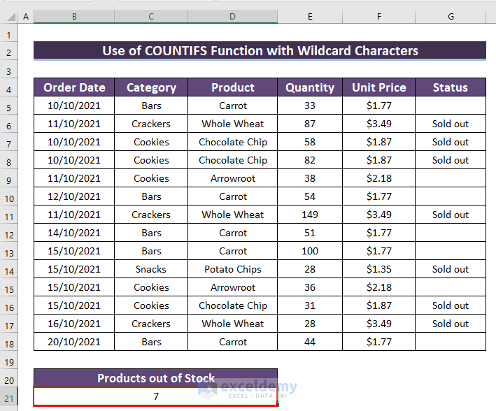
Example 4 – Using the COUNTIFS Function with Wildcard Characters
We can use Wildcard Characters such as “*”, “?” to check for the number of products out of stock.
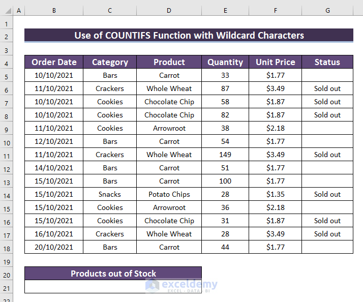
Steps:
- Use the following formula in the merged cells B21:D21.
=COUNTIFS($D$5:$D$18,"*",$G$5:$G$18,"<>"&"")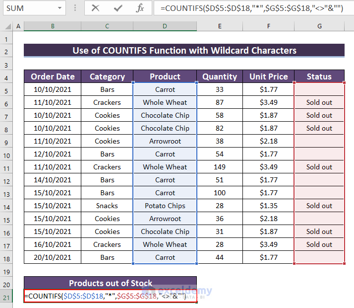
- Hit Enter.
Practice Section
You can download the Excel file and practice the methods.
Download the Practice Workbook
Excel COUNTIFS Multiple Criteria: Knowledge Hub
- Excel COUNTIFS Function with Multiple Criteria in Same Column
- Excel COUNTIFS with Multiple Criteria and OR Logic
- Excel COUNTIFS with Multiple Criteria Including Not Blank
- COUNTIFS Function in Excel with Multiple Criteria from Different Sheet
<< Go Back to Excel COUNTIFS Function | Excel Functions | Learn Excel
Get FREE Advanced Excel Exercises with Solutions!
