Excel COUNTIFS with Multiple Criteria Including Not Blank

Like the COUNTIF function, the COUNTIFS function counts the number where specified conditions are true. The difference between them is mainly that the former works on one condition while the latter can take multiple criteria. This article will focus on using the COUNTIFS function for not blank values with multiple criteria in Excel.

Download Practice Workbook

You can download the workbook used for the demonstration from the download link below.

How to Use COUNTIFS with Multiple Criteria Including Not Blank in Excel

The COUNTIFS function mainly counts the number of cells in one or more given arrays that maintain one or more specific criteria. The main syntax for the function is

So we can see the function takes a range and then a criterion of what to select from the range. Then it takes another range and criteria to pick from the second range. It can go on for multiple ranges and criteria. It finally returns the number of times all of the criteria match.

For non-blank values, the criteria are defined with an AND (&) operator. The syntax for the not blank criteria is “<>”&””. If we use it in criteria after a range, the COUNTIFS function will only include not blank values along with other multiple criteria for the Excel spreadsheet.

So the syntax for the COUNTIFS function for non-blank values must include the pair:

4 Examples to Use COUNTIFS with Multiple Criteria Including Not Blank in Excel

Now we will look at four different examples where we will utilize the COUNTIFS function as described above for multiple criteria which include not blank values in Excel. We will have different datasets for different examples. And in the end, we will focus on the breakdown of how each formula is working.

1. Counting Cells That Have a Pastime with Valid Birthday

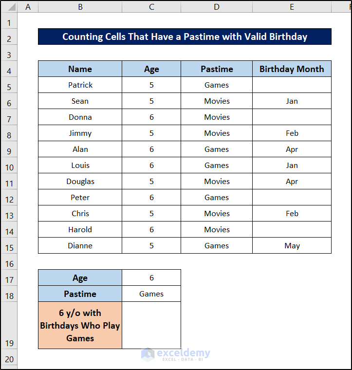
First, we will work with the following dataset.

Here, we can see there are some blank values in the “Birthday Month” Column. For the demonstration, we will focus on 6-year-old children who have games as their pastimes and have a birthday entry in the final column.

Follow these steps to see how we can do that with the COUNTIFS function.

Steps:

• First, let’s prepare the dataset for the purpose. We will put the desired values to compare in separate cells.

• Now select cell C19.
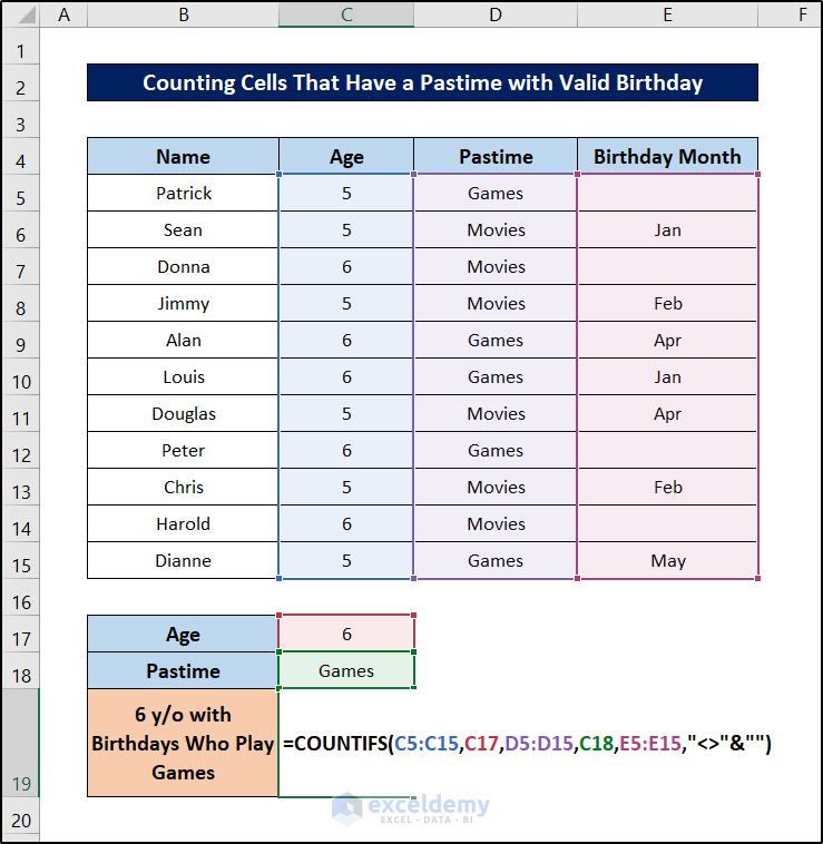
• Then write down the following formula in the cell.

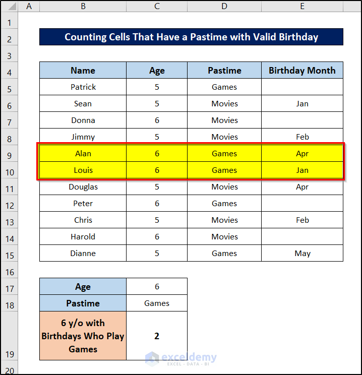
• After that, press Enter on your keyboard.

As a result, you will have the not blank values along with multiple criteria included in the COUNTIFS function in the Excel worksheet.

This is how you can use the COUNTIFS function for multiple criteria with not blank values in Excel.

Read More: Excel COUNTIFS Function with Multiple Criteria in Same Column

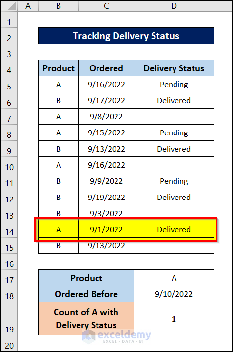
2. Tracking Delivery Status

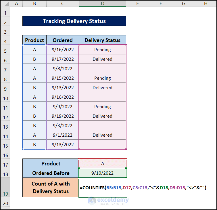
Next, we will demonstrate an example with the following dataset.

There are two products in the dataset along with the ordered date. In the final column, there are some missing values for the delivery status. Now we will pick out the values which have the delivery status for a specific product and before a specific date, say 10th September.

Follow these steps to see how we can do that.

Steps:

• First, let’s prepare the sheet for the desired values.

• Then select cell C19.
• After that, write down the following formula.

• Finally, press Enter. You will have the desired value.

This is another example of how we can use the COUNTIFS function for not blank values in one of the multiple criteria in Excel.

Read More: Excel COUNTIFS Not Working with Multiple Criteria (2 Solutions)

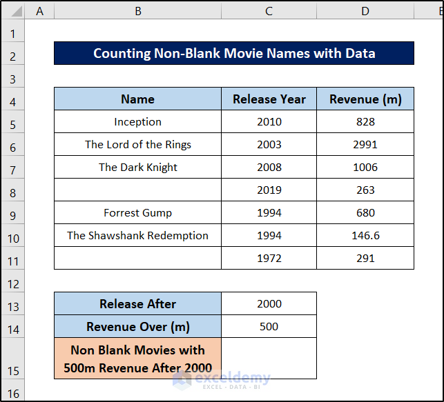
3. Count Non-Blank Movie Names with Data

In the previous two examples, we have used equal values and one unequal value with the COUNTIFS function as criteria along with the non-blank one. In this example, let’s try out double unequal criteria. First, let’s take a dataset.

Then follow these steps to see how we can use the COUNTIFS function for not blank values along with multiple criteria in Excel and count our desired results.

Steps:

• First, let’s prepare the values in separate cells.

• Then select the cell where you want to put the count value. Here, we are selecting cell C15.
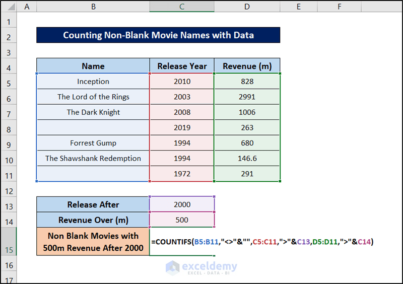
• After that, write down the following formula.

• Finally, press Enter. Thus you will have the count where the desired criteria are met.

Read More: How to Use COUNTIFS with Date Range and Text in Excel

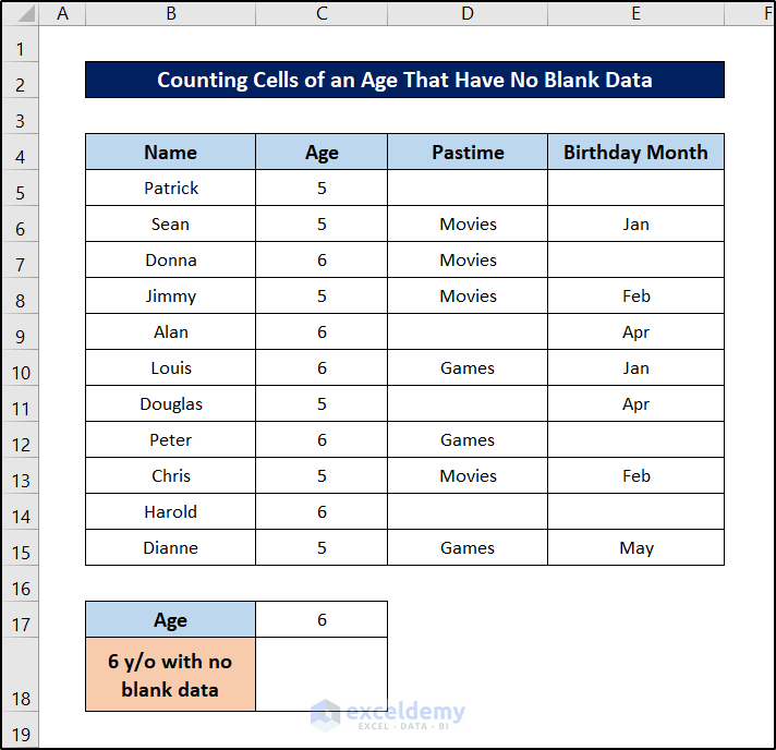
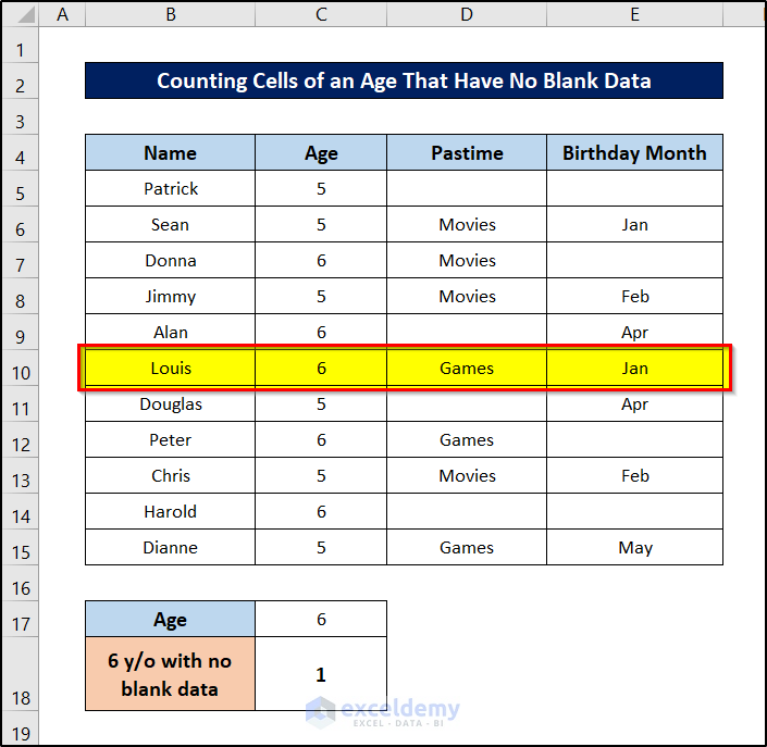
4. Counting Cells of a Particular Age That Have No Blank Data

Now let’s take a look at a different scenario. For the dataset in the first example, we are taking multiple blank values now.

In this example, we are going to use only non-blank criteria multiple times in the COUNTIFS function and find out rows that do not contain blank values in Excel.

Follow these steps to find out how we can do that.

Steps:

• First, prepare the cells to work with multiple criteria similar to the previous examples.

• Then select cell C18 and write down the following formula.

• Finally, press Enter on your keyboard.

This is how we can use the not blank criterion as multiple criteria in the COUNTIFS function in Excel and find rows that do not contain any non-blank values.

Read More: COUNTIFS Function in Excel with Multiple Criteria from Different Sheet

Conclusion

These were some of the examples of using the COUNTIFS function for not blank values with multiple criteria in Excel. Hopefully, you have grasped the usage of the function along with non-blank values and can use it accordingly to your scenario. I hope you found this guide helpful and informative. If you have any questions or suggestions, let us know in the comments below.

For more guides like this, visit Exceldemy.com.

Related Articles

• COUNTIFS to Count Across Multiple Columns in Excel
• Excel COUNTIFS with Multiple Criteria and OR Logic (3 Examples)