In this tutorial, I am going to show you 4 practical examples of how to use COUNTIFS with date range and text in Excel. You can quickly use these methods even in large datasets to count any specific criteria-based cells. Throughout this tutorial, you will also learn some important Excel tools and functions which will be very useful in any Excel related task.
How to Use COUNTIFS with Date Range and Text in Excel: 4 Practical Examples
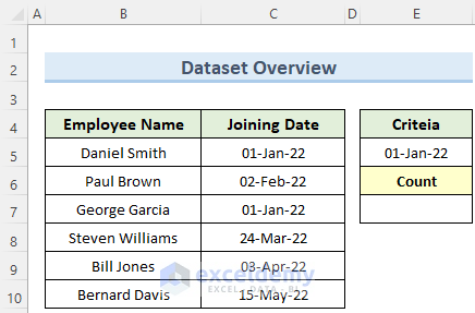
We have taken a concise dataset to explain the steps clearly. The Excel dataset has approximately 6 rows and 3 columns. Initially, we formatted all the cells containing date ranges in Date format. For all the datasets, we have 3 columns Employee Name, Joining Date, and Criteria. We have set the required criteria before beginning a method.
1. Counting Date Occurrence
One of the common ways to use the COUNTIFS function with date range and text is to count certain date occurrences. Let us see how we can achieve this.
Steps:
- First, go to cell E7 and insert the following formula:
=COUNTIFS(C5:C10,E5)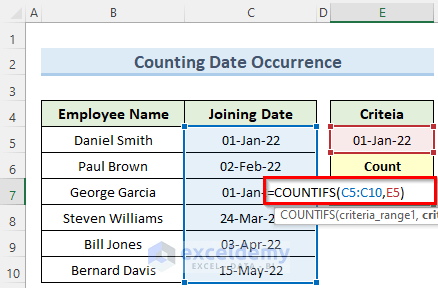
- Now, press the Enter key and you should see the number of times that date occurs inside cell E7.

2. Finding Year Occurrence
We can also find a specific year occurrence within a date range and text dataset. For this, we will use the DATE function alongside the COUNTIFS function. Follow the steps below.
Steps:
- To begin with, double-click on cell E7 and enter the below formula:
=COUNTIFS(C5:C10,">="&DATE(E5,1,1),C5:C10,"<="&DATE(E5,12,31))
- Next, press Enter and this will calculate the number of times the year 2021 occurs in the data range.

🔎 How Does the Formula Work?
- DATE(E5,1,1) : This portion returns the date as 01-Jan-2021.
- DATE(E5,12,31): This returns the date 31-Dec-2021.
- “>=”&DATE(E5,1,1),C5:C10,”<=”&DATE(E5,12,31): This returns the condition greater than 01-Jan-2021 and less than 31-Dec-2021.
Read More: Excel COUNTIFS Not Working with Multiple Criteria
3. Counting Cells Containing Certain Word
If we have a dataset with date range and text, then we can easily use the COUNTIFS function to count the number of cells with a specific word. See the steps below to do this.
Steps:
- To begin this method, double-click on cell E7 and insert the formula below:
=COUNTIFS(B5:B10,"*Daniel*")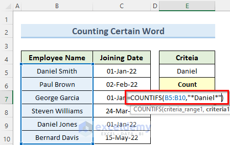
- Finally, press the Enter key or click on any empty cell to count the given word.

Read More: Excel COUNTIFS with Multiple Criteria Including Not Blank
4. Words Counting with OR Logic
In this final method, we will see how to use the COUNTIFS function to find any of the specified words within a dataset with date range and text. We will use the * sign for this purpose.
Steps:
- To start this method, navigate to cell E7 and type in the following formula:
=SUM(COUNTIFS(B5:B10,{"Daniel Smith","Paul Brown"}))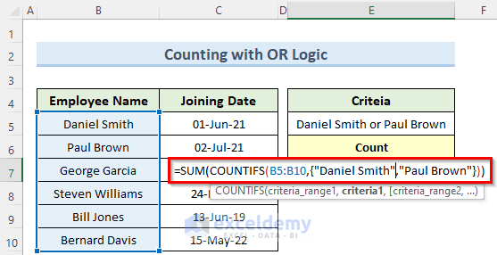
- Now, press Enter and you should get the number of times the criteria are found in the specific range.

Read More: Excel COUNTIFS with Multiple Criteria and OR Logic
Things to Remember
- Although we have used a single criteria cell for simplicity, you can use more if you need to.
- The COUNTIFS function can take multiple ranges and criteria, so you can work with that when needed.
- You can use up to 127 criteria.
- This function is not case-sensitive, so you may write the word Daniel as daniel.
- Remember to use the * wildcard character inside the formula, otherwise, it will not work.
- When you use non-numeric criteria inside the COUNTIFS function, you have to put double quotes around them.
- You can use the? mark instead of the * but it may not work in some cases.
Download Practice Workbook
You can download the practice workbook from here.
Conclusion
I hope that you were able to apply the above methods to use COUNTIFS with date range and text in Excel. Make sure to download the workbook provided to practice and also try these methods with your own datasets. If you get stuck in any of the steps, I recommend going through them a few times to clear up any confusion. If you have any queries, please let me know in the comments.
Related Articles
- COUNTIFS to Count Across Multiple Columns in Excel
- Excel COUNTIFS Function with Multiple Criteria in Same Column
- COUNTIFS Function in Excel with Multiple Criteria from Different Sheet
<< Go Back to Excel COUNTIFS Multiple Criteria | Excel COUNTIFS Function | Excel Functions | Learn Excel
Get FREE Advanced Excel Exercises with Solutions!
