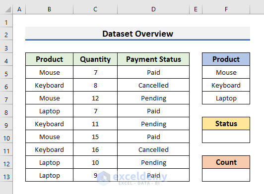
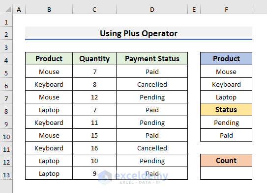
The sample dataset contains information about Products, their Payment Status and Quantity.
To count the number of laptops and keyboards with pending or paid status:
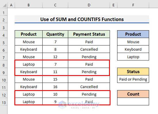
Example 1 – Using the SUM and COUNTIFS Functions with Multiple Criteria and the OR Logic
STEPS:
- Select F13 and enter the formula below:
=SUM(COUNTIFS(B5:B13,{"Laptop","Keyboard"},D5:D13,{"Paid";"Pending"}))- Press Enter to see the result.
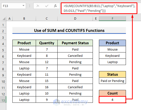
The criteria range and criteria were entered in the COUNTIFS function. The first criteria looks for a Laptop or Keyboard in B5:B13 and the second criteria looks for Paid or Pending in D5:D13.
Formula Breakdown
- COUNTIFS(B5:B13,{“Laptop”,”Keyboard”},D5:D13,{“Paid”;”Pending”}): This output is an array: {2,0,1,1}. It can be displayed as shown below:
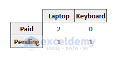
The number of Paid Laptops is 2 and Pending is 1. The number of Paid Keyboards is 0 and Pending is 1. The total number is 4.
- SUM(COUNTIFS(B5:B13,{“Laptop”,”Keyboard”},D5:D13,{“Paid”;”Pending”})): The SUM function adds the array {2,0,1,1} and displays the result: 4.
Example 2 – Applying the Excel COUNTIFS Function with the Plus Operator to Count Cells with Multiple Criteria
The dataset is slightly different.
To count the number of cells that contain Laptop and Keyboard with Paid or Pending status:
STEPS:
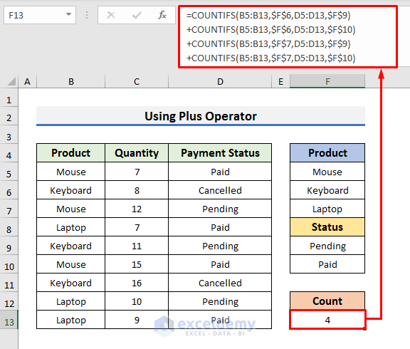
- Select F13 and enter the formula below:
=COUNTIFS(B5:B13,$F$6,D5:D13,$F$9)+COUNTIFS(B5:B13,$F$6,D5:D13,$F$10)+COUNTIFS(B5:B13,$F$7,D5:D13,$F$9)+COUNTIFS(B5:B13,$F$7,D5:D13,$F$10)- Press Enter to see the result.
An absolute cell reference was used.
Formula Breakdown
The formula is broken into four parts: each part counts the cell number specified by the condition.
- COUNTIFS(B5:B13,$F$6,D5:D13,$F$9): counts the number of cells that contain Keyboard in B5:B13 and Pending in D5:D13.
- COUNTIFS(B5:B13,$F$6,D5:D13,$F$10): counts the number of cells that contain Keyboard in B5:B13 and Paid in D5:D13.
- COUNTIFS(B5:B13,$F$7,D5:D13,$F$9): counts the number of cells that contain Laptop in B5:B13 and Pending in D5:D13.
- COUNTIFS(B5:B13,$F$7,D5:D13,$F$10): counts the cell numbers that store Laptop in B5:B13 and Paid in D5:D13.
- The Plus (+) operator sums the value and shows the result.
Read More: COUNTIFS Function in Excel with Multiple Criteria from Different Sheet
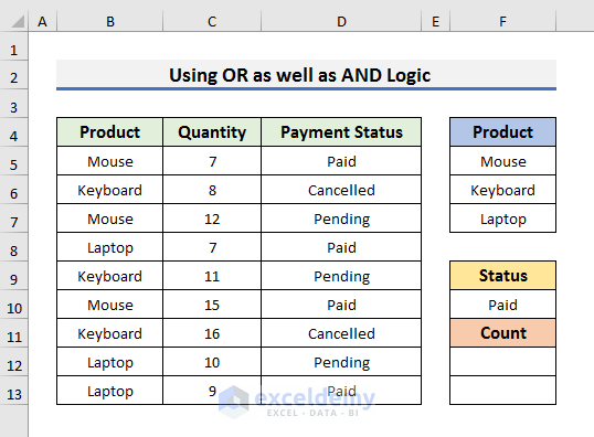
Example 3 – Counting Cells Using the Excel COUNTIFS Formula with the OR and the AND Logic
Count the number of cells that contain Laptop or Keyboard in B5:B13 and Paid in D5:D13:
STEPS:
- Select F12 and enter the formula below:
=COUNTIFS(B5:B13,F6:F7,D5:D13,F10)- Press Ctrl + Shift + Enter to see the result.
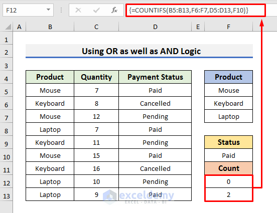
This formula is an array formula. {0,2} is the result.
- The first condition looks for Keyboard or Laptop in B5:B13.
- The second condition looks for Paid in D5:D13.
- To sum the array {0,2}, use the formula below:
=SUM(COUNTIFS(B5:B13,F6:F7,D5:D13,F10))
Alternative to the Excel COUNTIFS Function to Count Cells with Multiple Sets of OR Criteria
Consider the dataset in Example 1. To count cells that contain Laptop or Keyboard with the payment status Paid or Pending:
STEPS:
- Select F13 and enter the formula below:
=SUMPRODUCT(ISNUMBER(MATCH(B5:B13,{"Laptop","Keyboard"},0))*ISNUMBER(MATCH(D5:D13,{"Paid","Pending"},0)))- Press Enter to see the result.
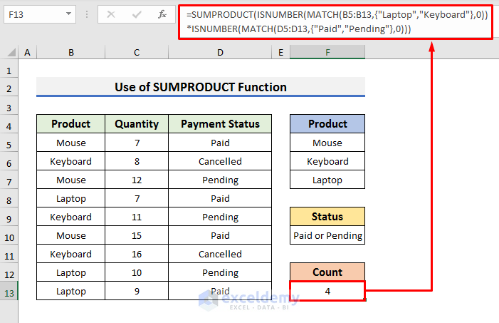
The MATCH function looks for the exact match in the selected range. The ISNUMBER function checks if the returned value is a number. If it is a number, it returns TRUE. Otherwise, FALSE.
Formula Breakdown
- MATCH(B5:B13,{“Laptop”,”Keyboard”},0): returns the array:
{#N/A, 2, #N/A, 1, 2, #N/A, 2, 1, 1}
- ISNUMBER(MATCH(B5:B13,{“Laptop”,”Keyboard”},0)): checks if the returned array contains a number. The output is:
{FALSE, TRUE, FALSE, TRUE, TRUE, FALSE, TRUE, TRUE, TRUE}
- ISNUMBER(MATCH(D5:D13,{“Paid”,”Pending”},0)): The output of this part is:
{TRUE, FALSE, TRUE, TRUE, TRUE, TRUE, FALSE, TRUE, TRUE}
- ISNUMBER(MATCH(B5:B13,{“Laptop”,”Keyboard”},0))*ISNUMBER(MATCH(D5:D13,{“Paid”,”Pending”},0)): multiplies the two arrays. The result becomes:
{0, 0, 0, 1, 1, 0, 0, 1, 1}
- The SUMPRODUCT function returns the sum of the products in the array: 4.
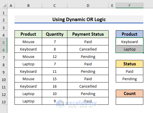
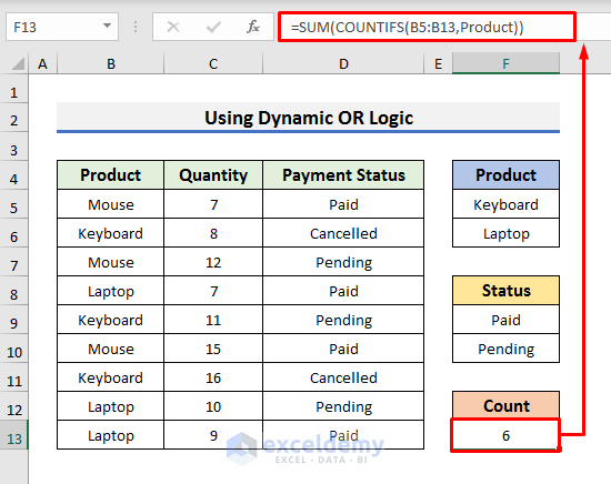
How to Apply the COUNTIFS Function with a Dynamic OR Logic in Excel
Count the number of cells that contain Laptop or Keyboard in B5:B13:
STEPS:
- Select F5:F6.
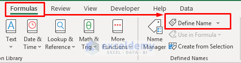
- Go to Formulas and select Define Name.
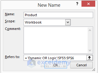
- Enter a name in Name (here, Product) and click OK.
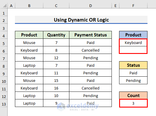
- Select F13 and use the formula below:
=SUM(COUNTIFS(B5:B13,Product))- Press Enter to see the result.
- If you remove the word Laptop from F6, the result in F13 will automatically update.
Read More: How to Use COUNTIFS with Date Range and Text in Excel
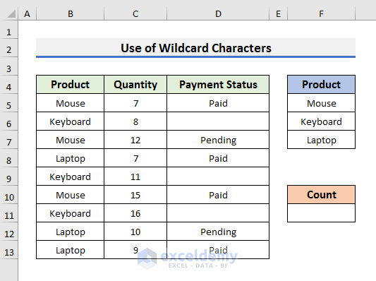
How to Use the COUNTIFS Function with Wildcard Characters in Excel
Consider the dataset below.
Count the number of cells with a displayed payment status.
STEPS:
- Select F11 and enter the formula below:
=COUNTIFS(B5:B13,"*",D5:D13,"<>"&"")- Press Enter to see the result.
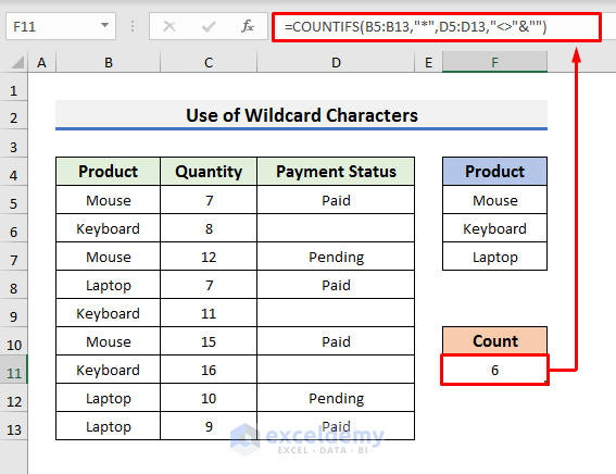
This formula matches B5:B13 with D5:D13 and finds non-empty cells.
Download Practice Workbook
Download the practice workbook.
Related Articles
- How to Use COUNTIFS to Count Across Multiple Columns in Excel
- Excel COUNTIFS with Multiple Criteria Including Not Blank
- Excel COUNTIFS Function with Multiple Criteria in Same Column
<< Go Back to Excel COUNTIFS Multiple Criteria | Excel COUNTIFS Function | Excel Functions | Learn Excel
Get FREE Advanced Excel Exercises with Solutions!
