This article will demonstrate comprehensively how the SUM function works in Excel, both on its own and in conjunction with other Excel functions.
Overview of the SUM Function
Summary
Adds all the numbers in given ranges of cells.
Syntax
=SUM (number1, [number2], [number3], ...)Arguments
| ARGUMENT | REQUIREMENT | EXPLANATION |
|---|---|---|
| number1 | Required | The first value to sum. |
| [number2] | Optional | The second value to sum. |
| [number3] | Optional | The third value to sum. |
Note:
- If arguments contain errors, SUM will throw an error.
- SUM automatically ignores empty cells and cells with text values.
- This function can take up to 255 total arguments.
- Arguments can be supplied as constants, ranges, named ranges, or cell references.
How to Use the SUM Function in Excel: 6 Examples
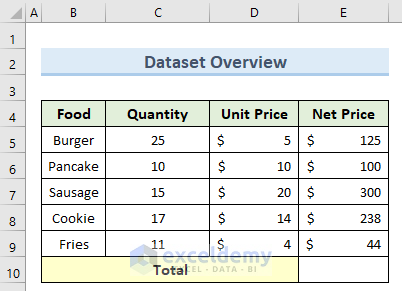
To explain our examples, we’ll use the following sample dataset. Initially, all the cells are in General format except the Price columns which are in Accounting format.
Example 1 – Summing a Range
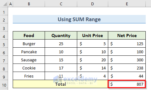
Let’s calculate the Total Net Price of all the items using the SUM function.
Steps:
- Enter the following formula in cell E10:
=SUM(E5:E9)
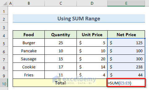
- Press Enter to perform the sum operation.
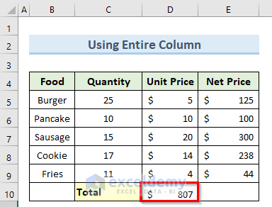
Example 2 – Summing an Entire Column
If we use a column as an argument, the SUM function will calculate the sum of all the numeric elements stored in that column.
Steps:
- Enter the following formula in cell D10:
=SUM(E:E)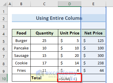
- Press Enter to get the column sum.
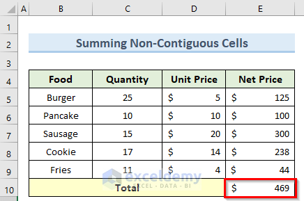
Example 3 – Summing Non-Contiguous Cells
Now let’s get the sum of some specific Total Price values by using their cell references as arguments in the SUM function.
Steps:
- Enter the following formula in cell E10:
=SUM(E5,E7,E9)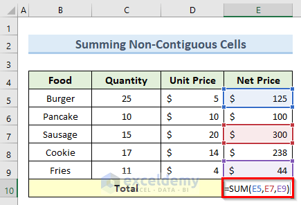
- Press Enter to perform the sum operation.
Read More: Excel SUM with OFFSET & MATCH Functions
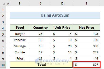
Example 4 – Using AutoSum Feature
Excel provides an option named AutoSum to make our calculations easier. Let’s use AutoSum to calculate the Total Net Price for our dataset.
Steps:
- Select cell E10.
- Go to the Formulas tab and click on AutoSum.
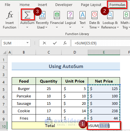
- Press Enter to return the sum of the values in the column above.
Example 5 – Summing Every Nth Row
Using the SUM function in the formula we can calculate the sum of every Nth row in a dataset. N could be 1,2,3,4……, etc. For example, let’s calculate the price sum of every third row in our dataset.
Steps:
- Enter the formula below in cell E10:
=SUM(E5:E9*(MOD(ROW(E5:E9),3)=0))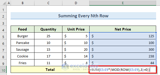
- Press Enter to return the sum for the specific criteria, or CTRL + SHIFT + ENTER if not using Office365.
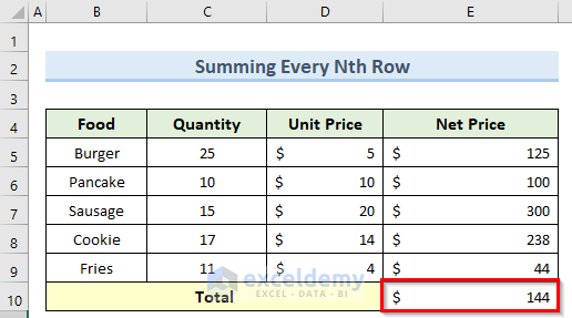
How Does the Formula Work?
- This is an array formula, which is why CTRL + SHIFT + ENTER is required for non-Office365 users.
- (MOD(ROW(E4:E12),3)=0): Finds the rows which are divisible by 3 (3, 6, 9 etc.) by using the ROW function.
- =SUM(E5:E9*(MOD(ROW(E5:E9),3)=0)): Sums the totals of the selected rows.
Example 6 – Summing the Largest Three Values
Suppose we want to find out the sum of the three top prices from the dataset.
Steps:
- Enter the formula below in cell E10:
=SUM(LARGE(E5:E9,{1,2,3}))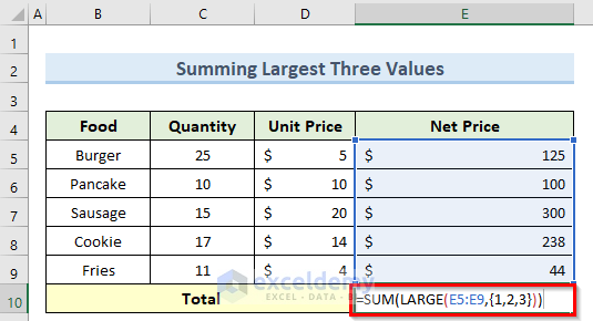
- Execute the sum by pressing the Enter key.
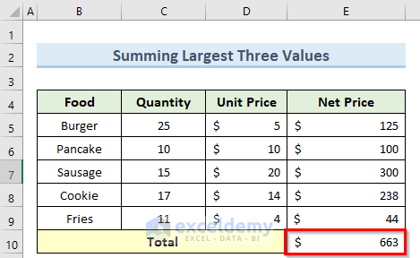
How Does the Formula Work?
- LARGE(E5:E9,{1,2,3}): The LARGE function returns the largest values from the E5:E9 range, and {1,2,3} defines the first 3 values in the selected data in that order, for example $500.00, $300.00, $242.00.
- SUM(LARGE(E5:E9,{1,2,3})): Calculates the sum of the selected three values.
Limitations of the SUM Function
- The cell range provided should meet the dimensions of the source.
- The cell including the output must always be formatted as a number.
Download Practice Workbook
<< Go Back to Excel Functions | Learn Excel
Get FREE Advanced Excel Exercises with Solutions!

HOW CAN I DO 1+1 IN EXCEL???
Hello Robert M,
You can simply type =1+1 into any Excel cell and press Enter. Excel will calculate it and show the result 2.
If you want to add values from cells, for example A1 and B1, you can type:
=A1+B1
This way, Excel will add the numbers inside those cells.
Regards,
ExcelDemy