How to Trigger Conditional Formatting Based on External Workbook Values

 

Conditional formatting based on external workbook values allows you to automatically format cells in one Excel workbook based on data stored in another workbook. This feature is essential to create dynamic reports, dashboards, and data comparisons across multiple files in business environments.

In this tutorial, we will show how to trigger conditional formatting based on external workbook values.

Let’s say you track actual quarterly sales in one file and quarterly sales targets in another. In the actuals sheet, you want to highlight any actual sales below target, pulling the correct targets from the external file.

Method 1: Helper Column with External Reference

This is the most reliable method that works in all Excel versions. You can use a worksheet formula with an external reference in a helper column. Apply conditional formatting based on the values of the helper column.

Step 1: Prepare Your Workbooks

First, create and save both workbooks with the sample data above:

• Create “Sales Target.xlsx” and enter the target data.
• Save it to your desktop or a specific folder.
• Create “Actual Sales.xlsx” and enter the actual sales data.
• Save it in the same location.

Step 2: Create Helper Columns with External References

• In “Actual Sales.xlsx”, add helper columns (starting in column G):
• Select cell G2 and insert the following formula.

=[SalesTarget.xlsx]Quarterly_Targets!B2

• Drag the formula right to autofill the formula in cells H2, I2, and J2.

• To update values, select the Sales Target.xlsx file.

• Select cell G2:J2.
• Drag the formula down to autofill the formula in the rest of the cells.

Step 3: Apply Conditional Formatting Using Helper Columns

Now use internal references for conditional formatting.

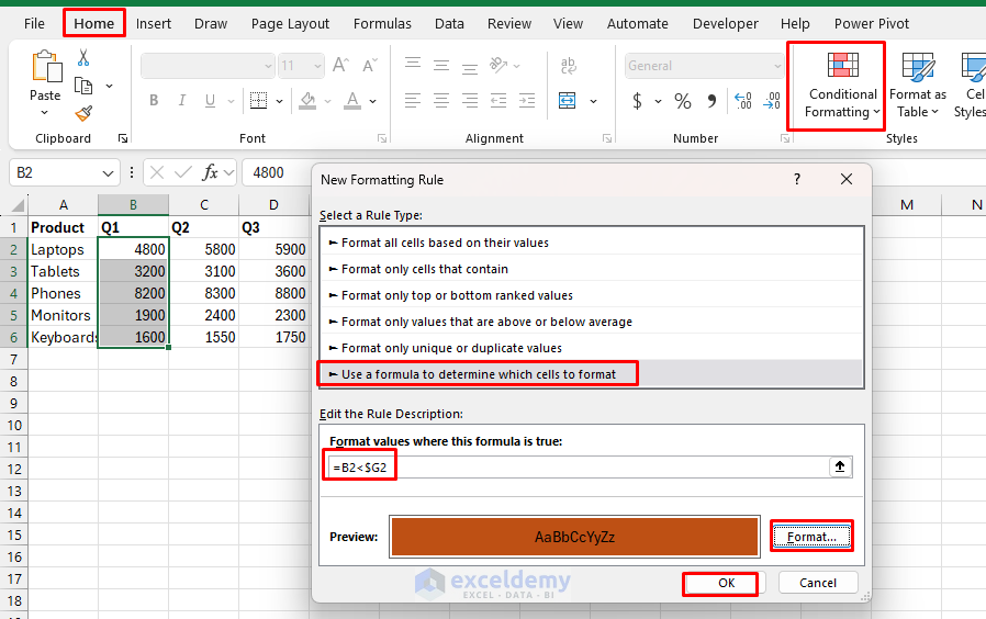
• Select the cell range (B2:B6).
• Go to the Home tab >> select Conditional Formatting >> select New Rule.
• Choose Use a formula to determine which cells to format.
• Enter the following formula:

=B2<$G2

• Click Format >> select Light red fill color.
• Click OK.

Add More Rules:

Repeat for each quarter as needed.

Quarter 2:

• Enter the following formula:

=C2<$H2

• Click Format >> select Light blue fill color.
• Click OK.

Quarter 3:

• Enter the following formula:

=D2<$I2

• Click Format >> select Light green fill color.
• Click OK.

Quarter 4:

• Enter the following formula:

=E2<$GJ2

• Click Format >> select Light purple fill color.
• Click OK.

Step 4: Hide Helper Columns (Optional)

• Select columns G:J.
• Right-click >> select Hide.

Your data will show conditional formatting based on external workbook values, but Excel uses internal helper columns to avoid the external reference limitation.

Method 2: Use Power Query Solution

Power Query provides a robust solution for users with Excel 365 or Excel 2016+.

Step 1: Import External Data with Power Query

• Open the “Actual Sales.xlsx” workbook.
• Go to the Data tab >> select Get Data >> select From File >> select From Workbook.
• Browse to select the “Sales Target.xlsx” file.
• Choose the “Quarterly_Targets” table.
• Click Import.

• In the Navigator window >> select the data sheet.
• Click Transform Data.

• In Power Query Editor:
  • Rename columns to match your needs (Target_Q1, Target_Q2, etc.).
  • Go to the Home tab >> Close & Load To.

• • Select Table >> select New worksheet.
  • Click OK.

Step 2: Apply Conditional Formatting

Now use standard conditional formatting with the imported data as in solution 1, but referencing only internal data.

• Select the cell range (B2:B6).
• Go to the Home tab >> select Conditional Formatting >> select New Rule.
• Choose Use a formula to determine which cells to format.
• Enter the following formula:

=B2 <Quarterly_Targets!$B2

• Click Format >> select Light red fill color.
• Click OK.

• Add more rules for the rest of the quarters.

Quarter 2:

=C2 <Quarterly_Targets!$C2

Quarter 3:

=D2 <Quarterly_Targets!$D2

Quarter 4:

=E2 <Quarterly_Targets!$E2

• Refresh Power Query anytime the targets change.
  • Right-click >> select Refresh.
• You can schedule an automatic refresh if your data changes frequently.
• Go to the Data tab >> select Queries and Connections.
• Right-click on the Queries >> select Properties.

• In Refresh every >> insert 5 minutes.
• Click OK.

This method automatically refreshes external data and avoids reference limitations.

Method 3: VBA Macro for Full Automation

If you’re comfortable with VBA, you can create a macro that updates conditional formatting based on external data. It will compare actuals and targets, applying formatting automatically, even if the reference file is closed.

To open the VBA Editor:

• Open your Actual Sales workbook.
• Go to the Developer tab >> select Visual Basic. Or press Alt + F11.
• In the Project window, right-click your workbook,
• Choose Insert >> select Module.

• Copy-paste the following VBA code.

VBA Code:

Sub HighlightSalesBelowTarget()
    Dim targetFilePath As String
    targetFilePath = "C:\Users\Sales Target.xlsx" ' <--- Update this to your file path
    
    Dim wbTarget As Workbook
    Dim wsTarget As Worksheet
    Dim wsActual As Worksheet
    Dim i As Long, j As Long
    Dim salesValue As Variant, targetValue As Variant
    
    Set wsActual = ThisWorkbook.Sheets("Performance_Data")
    Set wbTarget = Workbooks.Open(targetFilePath, ReadOnly:=True)
    Set wsTarget = wbTarget.Sheets("Quarterly_Targets")
    
    ' Data rows: 2 to 6, columns: 2 (B/Q1) to 5 (E/Q4)
    For i = 2 To 6         ' Rows: products
        For j = 2 To 5     ' Columns: Q1-Q4
            salesValue = wsActual.Cells(i, j).Value
            targetValue = wsTarget.Cells(i, j).Value
            If IsNumeric(salesValue) And IsNumeric(targetValue) Then
                If salesValue < targetValue Then
                    wsActual.Cells(i, j).Interior.Color = RGB(255, 199, 206)   ' Light red
                Else
                    wsActual.Cells(i, j).Interior.Pattern = xlNone             ' No color
                End If
            End If
        Next j
    Next i

    wbTarget.Close SaveChanges:=False
    MsgBox "Highlighting complete.", vbInformation
End Sub

• Update the file path with the full path to your Sales Target file.
• The macro opens the target workbook.
• Loop through each product and each quarter.
• If the sales value is less than the target, the cell is highlighted in light red.
• Macros close target workbooks automatically.

Save and Run:

• Save your workbook as a macro-enabled file (.xlsm).
• Go to the Developer tab >> select Macros.
• Select HighlightSalesBelowTarget >> click Run.

Output:

What Does NOT Work: Direct External References & Named Ranges

Some versions of Excel display the warning “You may not use references to other workbooks for Conditional Formatting criteria.”

• Direct external workbook references (e.g., =[Sales_Targets.xlsx]Quarterly_Targets!B2) are not allowed in conditional formatting rules. Excel will throw an error.
• Named ranges defined in the external workbook cannot be referenced in another workbook’s conditional formatting.
• Even using INDIRECT or similar functions will not work across files in this context.

There is no direct, native way to use external values in conditional formatting rules.

Recommendations

• For most businesses: Use Power Query to import external data. It is robust, supports refresh, and keeps all logic inside one workbook.
• For ad-hoc or quick checks: Use helper columns with external references if you do not mind keeping both files open.
• For automated, ongoing solutions: Use VBA for hands-off automation and formatting, especially for larger datasets.

Conclusion

External conditional formatting is a powerful feature that enables dynamic, cross-file data visualization. You can use any of the methods of your choice based on your scenario and convenience. Remember to always test your setup thoroughly and maintain clear documentation of external dependencies for future reference and collaboration with team members.

Triggering conditional formatting based on values from an external workbook is not possible natively in Excel.