In this article, we will explain what arrays are, what an array formula is, and provide several examples of how to use array formulas in Excel.
Introduction to Arrays in Excel
Before delving into array formulas, let’s consider what an array is in Excel.
Generally, an array is a group of things called elements. The elements may take the form of text or numeric values, which can be placed in a single row, a single column, or numerous rows and columns.
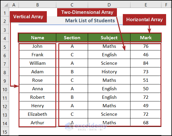
In the image above, two types of arrays are shown: one-dimensional (in a single row or column) and two-dimensional (across multiple rows and columns). One-dimensional arrays can further be differentiated into two sub-types: horizontal (in a row) and vertical (in a column).
Basics of Array Formulas
An array formula differs from a standard formula in that it handles numerous items as opposed to a single value. In other words, a formula for an array in Excel examines each value in the array individually and executes several computations on a single or a group of items in accordance with the conditions stated in the formula. There are two types of array formulas:
- One that returns the result in a single cell
- One that returns the output as an array.
We utilize array formulas in Excel for analysis of data, sums with criteria and different types of lookups, linear algorithms, calculation of matrices, and many other uses.
Array Formulas in Excel: 5 Examples
Now let’s work through some examples using array formulas in Excel.
Consider the dataset below containing the Mark List of Students of a certain institution. This dataset includes the Names of the students, and their corresponding marks in Maths and Science in columns B, C, and D respectively.
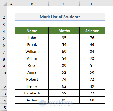
We’ll use this dataset to illustrate our first two examples.
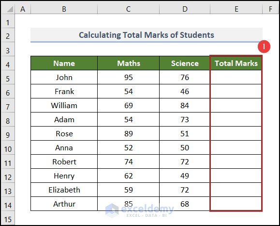
Example 1 – Calculating the Total Marks of the Students
Steps:
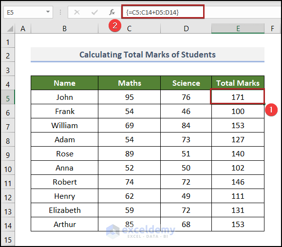
- Create a new column called Total Marks in Column E.
=C5:C14+D5:D14
- Press ENTER.
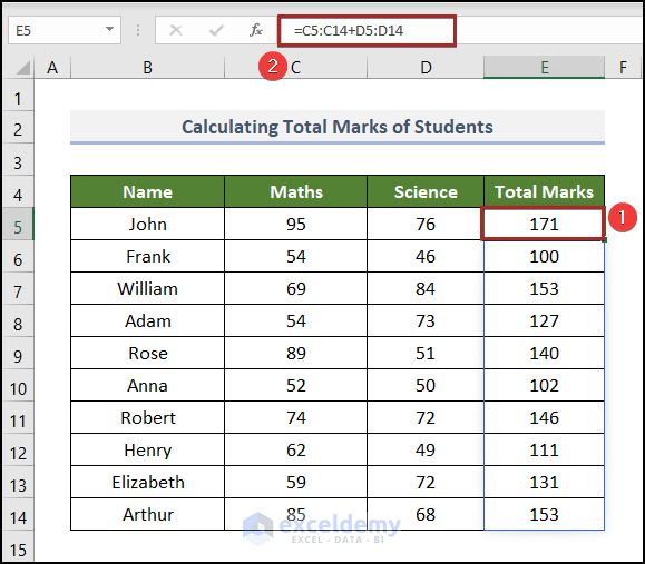
Note: Notice the light blue line around the cells in Column E. It signifies that these cells are in an array.
If you’re using Microsoft Excel 365 version, you can run an array formula by pressing ENTER. But in older versions of Excel, CTRL + SHIFT + ENTER must be used to run an array formula.
- Go to cell E5 and enter the same formula.
- Press CTRL + SHIFT + ENTER.
Note: After pressing this key combination, a pair of curly brackets will automatically be applied around the formula. You don’t need to enter them manually.
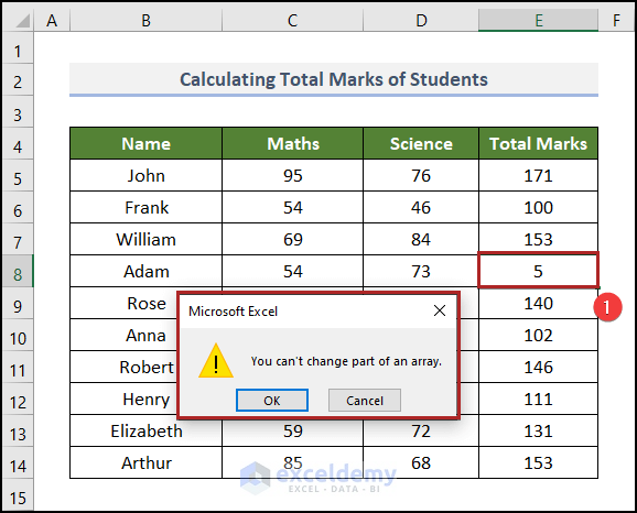
Also, we can’t make any changes inside a cell of an array.
- Go to cell E8 and change the value to 5.
- Press ENTER.
A warning box will be displayed like in the image below.
Example 2 – Determining the Highest Marks Obtained
Now let’s calculate the highest marks obtained by a student in any of the two subjects.
Steps:
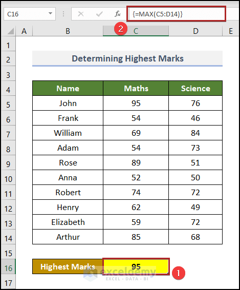
- Make an output range in cells B16:C16.
- Select cell C16 and enter the formula below:
=MAX(C5:D14)
Here, the MAX function returns the maximum value within the numbers in this range.
- Press ENTER.
Example 3 – An Array Formula with Multiple Criteria
Now we’ll demonstrate an array formula that will return a two-dimensional array with multiple criteria.
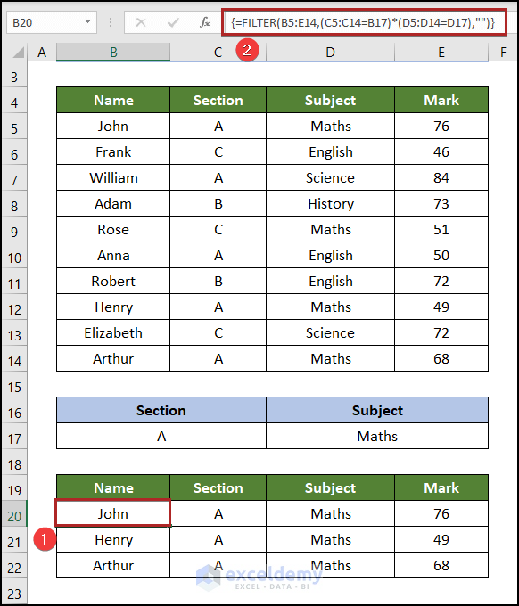
Our sample dataset contains the Name, Section, Subject, and Mark in columns B, C, D, and E consecutively. Also, we have Section A and Maths as the Subject in the B16:E17 range.
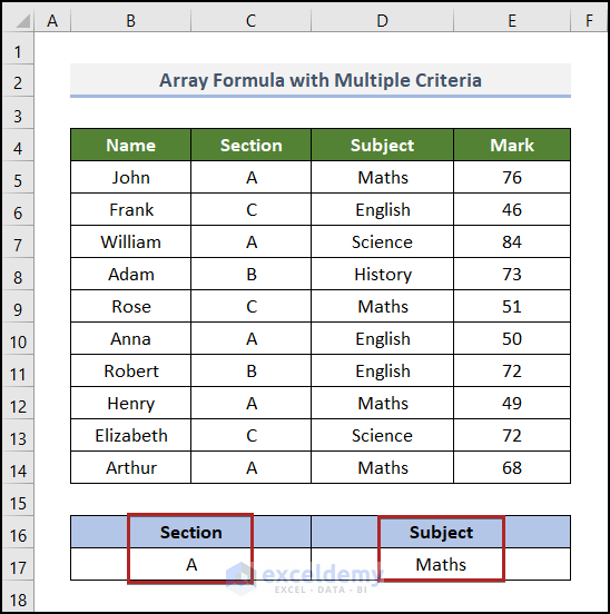
Now, we’ll filter the array in the B5:E14 range by the two criteria in the B16:E17 range, Section, and Subject.
Steps:
- Copy the headings in the B4:E4 range and paste them into the B19:E19 range.
- In cell B20 paste the following formula:
=FILTER(B5:E14,(C5:C14=B17)*(D5:D14=D17),"")
Here, B5:E14 represents the range of the array, C5:C14 represents the Section column, B17 is the section to be filtered, D5:D14 represents the Subject column, and D17 acts as the subject to be filtered.
The FILTER function has three arguments. Here, B5:E14 is the array argument and (C5:C14=B17)*(D5:D14=D17) is the include argument. This essentially works like a Boolean array; it carries the condition or criteria for filtering. In this case, we have two criteria combined by a (*) sign.
- Press ENTER.
Example 4 – Calculating Total Cost based on Quantity
Here, in Column B we have the Quantity of Unit. and in Column C is the corresponding Unit Price. We want to know the cost if we order a certain quantity of units.
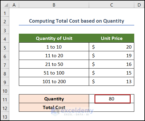
The unit price decreases gradually as the order amount increases. So, it costs less per unit if we order in bulk.
Steps:
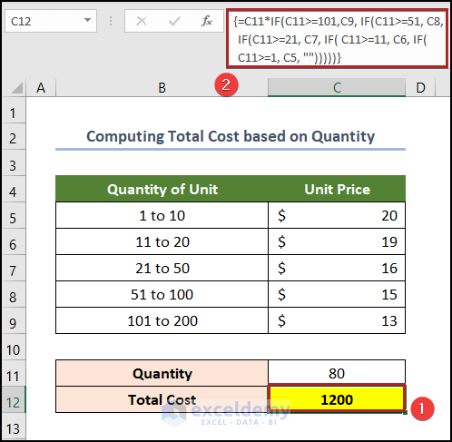
- In cell C12 enter the following formula:
=C11*IF(C11>=101,C9, IF(C11>=51, C8, IF(C11>=21, C7, IF( C11>=11, C6, IF(C11>=1, C5, "")))))
- IF(C11>=1, C5, ” “) →The IF function checks whether a condition is met, and returns one value if TRUE and another if FALSE. Here, C11>=1 is the logical_test argument which compares the value of cell C11 with 1. If the value is greater than or equal to 1 then the function returns the value of cell C5 (the value_if_true argument), otherwise it returns blank (the value_if_false argument).
- Output → 20
- IF( C11>=11, C6, IF(C11>=1, C5, “”)) → becomes IF( C11>=11, C6, 20).
- Output → 19
- IF(C11>=21, C7, IF( C11>=11, C6, IF(C11>=1, C5, “”))) → becomes IF(C11>=21, C7, 19).
- Output → 16
- IF(C11>=51, C8, IF(C11>=21, C7, IF( C11>=11, C6, IF(C11>=1, C5, “”)))) → becomes IF(C11>=51, C8, 16).
- Output → 15
- IF(C11>=101,C9, IF(C11>=51, C8, IF(C11>=21, C7, IF( C11>=11, C6, IF(C11>=1, C5, “”))))) → becomes IF(C11>=101,C9, 15).
- Output → 15
- C11*IF(C11>=101,C9, IF(C11>=51, C8, IF(C11>=21, C7, IF( C11>=11, C6, IF(C11>=1, C5, “”))))) → becomes C11*15.
- Output → 80*15 → 1200
- Press ENTER.
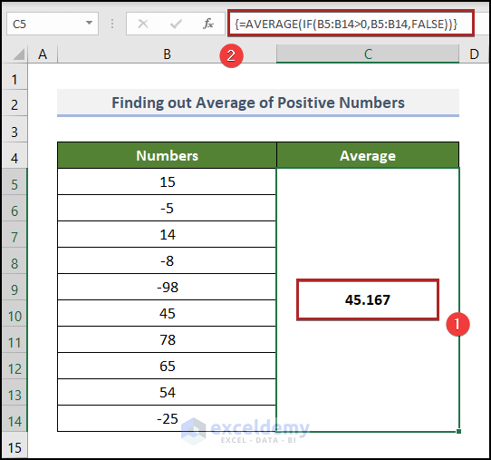
Example 5 – Calculating the Average of the Positive Numbers
In this worksheet, there are some numbers in Column B. Some are positive, and some are negative. Let’s determine the average of the positive numbers only in this range.
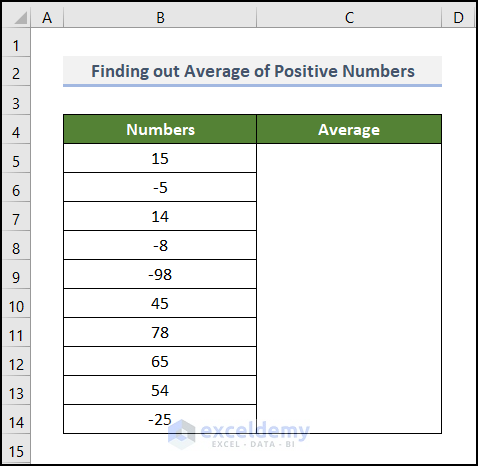
We can accomplish this in two ways. The first way is to separate the positive numbers manually, create a new range, and then use the AVERAGE function to find out the average of the positive numbers. A more efficient way is to use an array formula, which will save us time and effort.
Steps:
- In cell C5 enter the following formula:
=AVERAGE(IF(B5:B14>0,B5:B14,FALSE))
In an IF function, if the first argument of the function is TRUE then the second argument is returned. If the first argument is FALSE then the third argument is returned. Arguments are separated by commas.
In this case, the third argument is FALSE, so if the first argument is FALSE then the IF function will return the FALSE statement. The first argument is a range, as is the second argument, and the whole formula is an array formula.
- IF(B5:B14>0,B5:B14,FALSE) → Excel will create an array internally with the positive numbers and False statements.
- Output → {15, FALSE, 14, FALSE, FALSE, 45, 78, 65, 54, FALSE}
- AVERAGE(IF(B5:B14>0,B5:B14,FALSE)) → becomes AVERAGE({15, FALSE, 14, FALSE, FALSE, 45, 78, 65, 54, FALSE}).
- Output → 45.167
The AVERAGE function finds out the average of the values in the array, except for the FALSE values which are not numbers and therefore ignored.
- Press ENTER.
So, this is how an array formula works. The formula starts with the opening curly bracket and closes with the ending curly bracket, so we can observe that this is undoubtedly an array formula. As discussed above, the curly brackets are applied on an array formula automatically by Excel when we press CTRL, SHIFT, and ENTER.
What to Do If an Array Formula Is Not Working
If you are using a version of Excel older than the Excel 2019 version, you must press CTRL + SHIFT + ENTER to use the array formula. If you just press ENTER, your array formula will not work except in the case of a few functions such as the AGGREGATE and SUMPRODUCT functions.
Things to Remember
- You cannot construct an array with an entire column or multiple columns. This will hog system resources and can cause malfunctioning of the system.
- Use the F9 key to debug any part of an array formula. This makes it easy to evaluate.
- You need not place the curly brackets yourself; Excel will add them automatically.
- You can’t make any changes to a cell in an array. If you need to change a value, either edit the formula, or delete and recreate it in your preferred way.
Related Articles
<< Go Back to Array Formula | Excel Formulas | Learn Excel
Get FREE Advanced Excel Exercises with Solutions!

Big-time Thank You!
I am finally starting to “get it”! So many texts and web helper sites seem to be speaking either to infants or to PHDs. Your tone and style is simple without being inane. Interesting without being unnecessarily complicated. Great job!
Many thanks, Scott!
This is in awesome website and you are much more awesome Kawser!!!. I m loving excel now and will refer this to my friends too!!!. I will request you to plz share a practice worksheet containing advance excel problems for self practice. You should share the solutions on periodic basis. Thanks
It’s a good idea, Rahul. I will think about it soon.
Best regards
Kawser
Really straight forward and easy to understand… I am off to search for more of these array posts from you. Excited to see which is next!
Hello Jay, thanks for your nice words. Please visit our blog for more array posts! We have written more posts like this time by time.
Thank you very much for this tutorial, very useful in understanding what an array is and how it works in Excel.
You are welcome, Surya! 🙂
Excellent
Thank you so much, Ferreira. Visit our blog and explore more!
Hi
Got your “Excel Array Formula Basic 2 – Breakdown of Array Formula” great.
Question what is the name or address of Basin1
This would help me with Array Formula.
Bill
Hi Bill Coriell! Sorry for being late in reply. Maybe you were asking for the following article.
https://www.exceldemy.com/what-is-an-array-in-excel/
With regards
-ExelDemy team