How to Use Dynamic Arrays in Excel (20 Useful Functions)

Dynamic arrays in Excel help handle data without the need for complex formulas or manual adjustments. With the help of dynamic array formulas, you can quickly get the expanded required data in your Excel spreadsheet.

Today in this article, I am sharing how to use dynamic arrays in Excel using 20 functions with proper examples and illustrations.

In the following, you will find an overview of how to use dynamic arrays in Excel.

Download Practice Workbook

What Are Dynamic Arrays in Excel?

Dynamic arrays provide you with the result of generating all the output data at once. Unlike traditional Excel functions that return a single result, dynamic arrays can spill their results across adjacent cells. This simplifies complex calculations, accelerates data analysis, and makes managing dynamic datasets more efficient. Traditionally for dynamic calculation, we pressed CTRL+SHIFT+ENTER to get the dynamic range outputs. But now in Excel 365 you just need to press ENTER to get the final result.

In the following image you will see with just a single dynamic array formula we got all the output reducing time and complexity.

How to Use Dynamic Arrays in Excel: 20 Dynamic Array Functions

Suppose we have a dataset of some Salesperson, Product, Region, and their Selling Price in an Excel worksheet. Now we will use dynamic array formulas to get the required data with a single click.

Dynamic array functions are a set of powerful formula tools introduced with the release of Excel 365 and Excel 2021 for Windows and Mac. These functions provide dynamic arrays to automatically spill their results across multiple cells. Without moving here and there let’s get introduced to these functions.

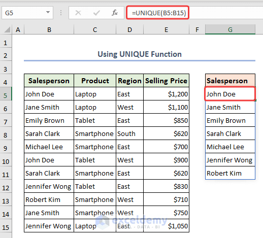
1. Using UNIQUE Function

The UNIQUE Function in Excel is used to get the unique values from a list of tables. Here we used the UNIQUE function to collect all the unique names providing the dynamic range.

• Simply, choose a cell (G5), apply the below formula, and hit ENTER.

• This way we will get all the unique names in the new column without dragging the Fill Handle confirming the dynamic feature in Excel.

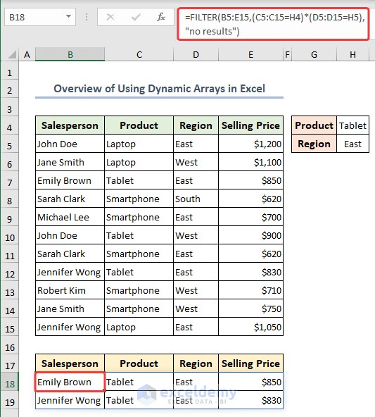
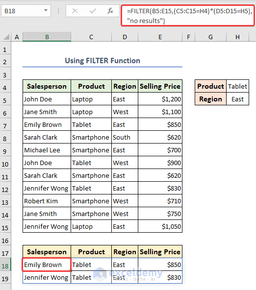
2. Applying FILTER Function

In order to filter data previously we had to type the complex formula and then drag the fill handle to get the result for multiple cells. But now you can insert the range in an array and get the result with a single formula. Isn’ it easy? In this part, we used the FILTER function to get the filtered data according to the criteria from the table.

• Select a cell (B18), write the following formula, and click ENTER.

• As a result, we got the filtered data from the table with a single formula.

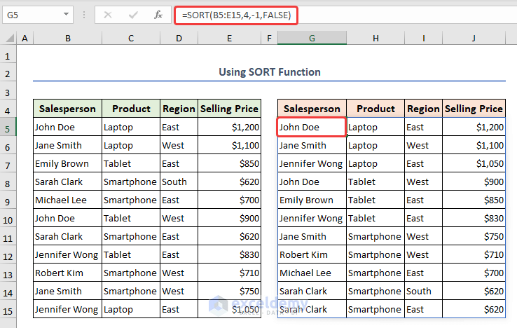
3. Inserting SORT Function

With the proper utilization of dynamic arrays, you can use the SORT function in Excel to sort the whole dataset according to ascending or descending order.

• Here we will sort the selling prices in descending order. First, choose a cell (G5), insert the below formula, and press ENTER.

• In conclusion, we have successfully got the sorted selling price in descending order. Simple isn’t it?

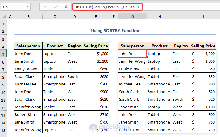
4. Applying SORTBY Function

The SORTBY function sorts the contents of a range or array based on the values in a corresponding range or array.

• Choose a cell (G5), apply the below formula, and click ENTER to get the result.

• Finally, we will get the result by sorting multiple columns from the table. In this part, first, we sorted the region in ascending order and then the selling price in descending order.

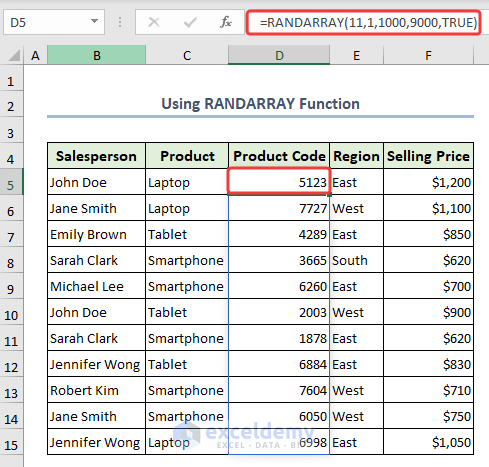
5. Using RANDARRAY Function

If you want you can also collect random values within the provided range and columns with a single click. Simply, use the RANDARRAY function to get random numbers for multiple cells.

• Start with choosing a cell (D5), write the following formula, and finish by hitting ENTER.

• In summary, we will get the random numbers generated for the chosen cells for product ID with a single formula.

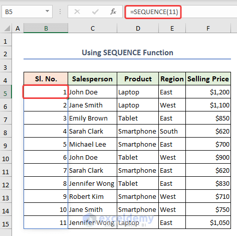
6. Using SEQUENCE Function

Previously, we used to insert sequential numbers and then Flash Fill to fill cells with sequential numbers. With dynamic array functions like the SEQUENCE function in Excel, we can directly get the sequence numbers for multiple cells. In this section, we created sequence numbers starting from 1 to 11 in the Sl. No. column.

• Choose a cell (B5), write the following formula, and hit ENTER key from the keyboard.

• Within a moment, our sequence numbers will be in our hands.

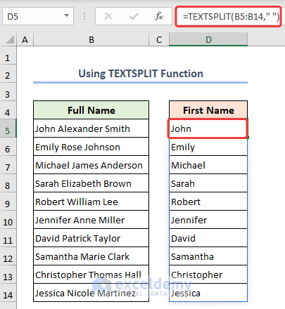
7. Inserting TEXTSPLIT Function

For splitting texts to multiple cells you can use the TEXTSPLIT function in Excel. In this method, we split the first name from the full name column.

• In the same fashion, choose a cell (D5), apply the formula, and click ENTER.

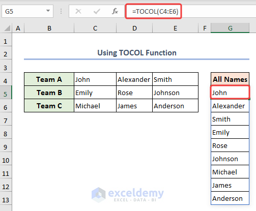
• That’s it, you will see the texts are split extracting all the first names from the column.

8. Applying TOCOL Function

In recent, Excel has introduced the TOCOL function which is mainly used to convert multiple data from rows to a single column.

• To combine the data in column G from three rows, we used the following formula.

• Within a blink of an eye, we will get all the data rearranged in a single column. Simple isn’t it?

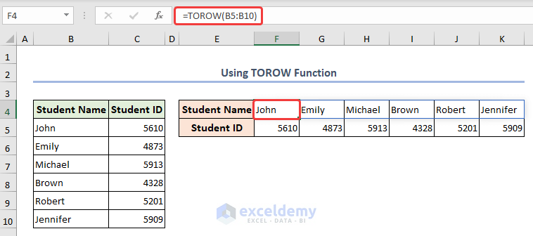
9. Applying TOROW Function

Well, the TOROW function works the same as the TRANSPOSE function in Excel. But for disorganized data, we recommend using the TOROW function in Excel.

• From the spreadsheet choose a cell (F4), write the formula, and hit ENTER.

• Finally, we have the range of data arranged row-wise. Here we organized the Student Names and IDs from column-wise to row-wise.

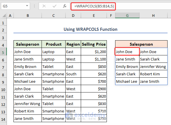
10. Applying WRAPCOLS Function

In order to wrap and group data to multiple columns you can try the WRAPCOLS function. Here, we’ll divide the name column into columns each column will have 5 names.

• Start with choosing a cell (G5), writing the formula, and clicking ENTER.

• Within a glimpse, we will get the names grouped from a single column to multiple cells.

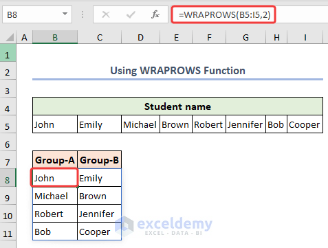
11. Using WRAPROWS Function

Just like the previous method, you can use the WRAPROWS function to rearrange rows of data into multiple groups.

• In this section, we made two groups each consisting of 4 names from the Student Name row. For this, choose a cell (B8), write the formula, and hit ENTER.

• In conclusion, we have successfully grouped and rearranged multiple names from the list.

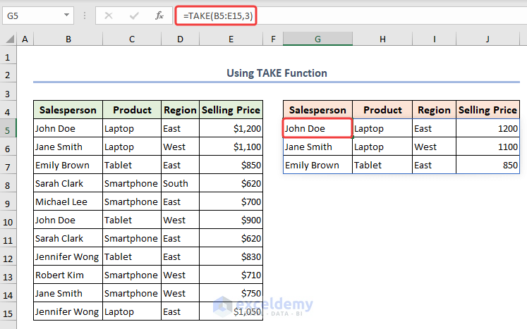
12. Inserting TAKE Function

In order to rearrange data according to your choice of group of cells you can try the TAKE function in Excel.

• Just choose a cell (G5), apply the formula, and hit ENTER.

• Finally, you will see that the function has returned the first three rows as an array.

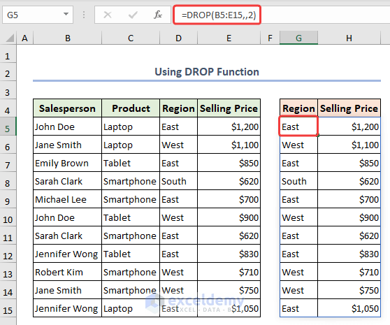
13. Inserting DROP Function

Sometimes copying and placing data into multiple locations seems monotonous work. Well, with the help of the DROP function, you can directly copy multiple columns and rows with a single formula.

• From the whole range of data, we copied the Region and Selling Price column to a new location. Thus, select a cell (G5), type the formula, and hit ENTER.

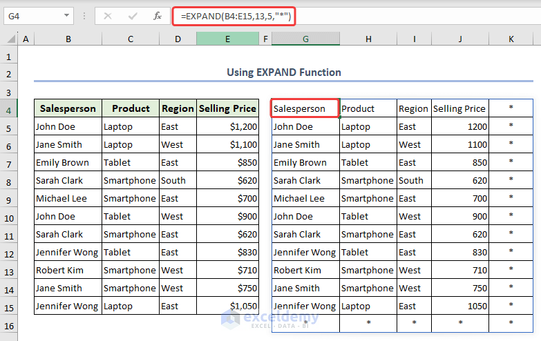
• Within a moment, according to the command of the formula, the data will be copied to the chosen location.

14. Applying EXPAND Function

The EXPAND function increases a cell range or array by a given number of rows and columns in an Excel spreadsheet.

• Choose a cell (G4), place the following formula, and click ENTER.

• In conclusion, we will see the data has expanded both row and column-wise. As you can see we used 13 inside the formula as we want to expand the rows to 13th. Similarly, inserted 5 columns starting from the left. And placed asterisk (*) in the last argument to return it in the expanded cells.

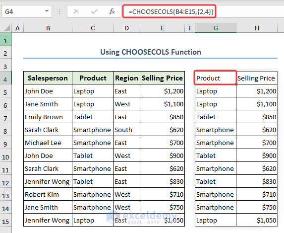
15. Using CHOOSECOLS Function

Sometimes copying non-adjacent columns from a large dataset might seem a tough one. But with proper use of the CHOOSECOLS function, you can copy multiple columns easily.

• Here, we will copy the 2nd and 4th columns from the table. Thus, select a cell (G4), write the below formula, and press ENTER.

• In summary, we will get the columns placed in a new place in the spreadsheet.

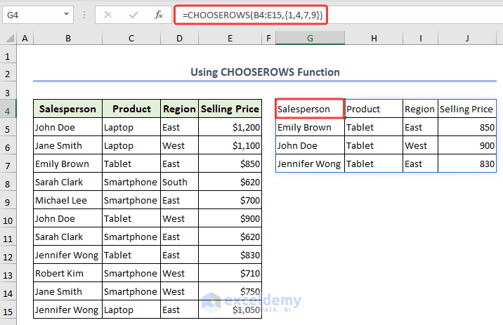
16. Applying CHOOSEROWS Function

Are you looking for a solution where you can copy multiple non-adjacent rows with only one formula? Well, you are at the right place where we will use the CHOOSEROWS function to copy multiple rows to a new location.

• Choose a cell (G4), apply the formula from below, and press ENTER.

• Finally, the chosen rows 1, 4, 7, and 9 will be copied to a new place with just a single click. It’s that simple.

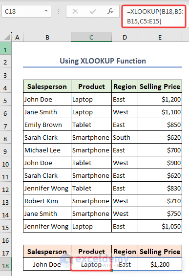
17. Using XLOOKUP Function

The XLOOKUP function allows you to search for values in dynamic arrays. Here in this part, we searched for all the values with the provided criteria which is the Salesperson named John Doe.

• Simply, choose a cell (C18), write the below formula, and press ENTER.

• Thus we will get all the values from the table matching the criteria. Look, there are two John Doe, XLOOKUP will return the first match.

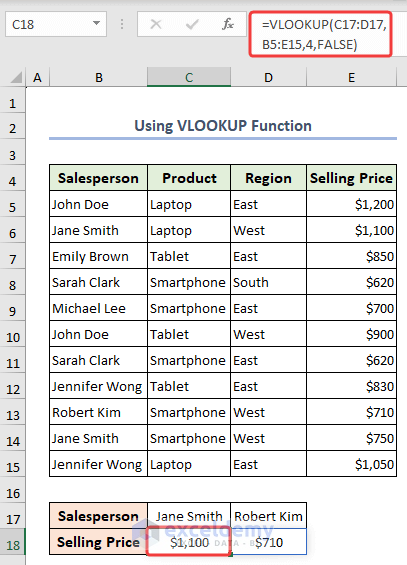
18. Applying VLOOKUP Function

The VLOOKUP function in Excel is a powerful and widely-used lookup function that stands for vertical lookup. Here, we will use the VLOOKUP function with multiple lookup values which are salesperson to collect their product’s selling price.

• For this, choose a cell (C18), write the below formula, and click ENTER.

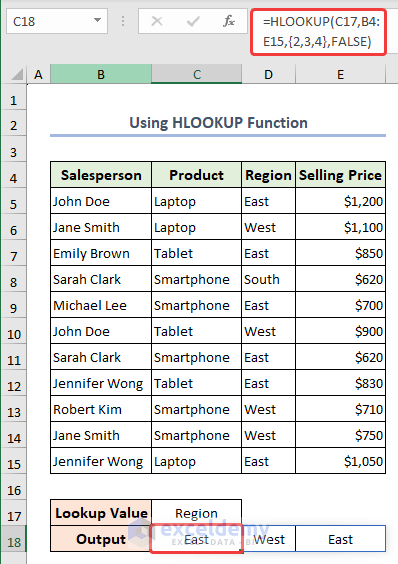
• As a result, we will get both the selling prices for the provided salesperson.

19. Inserting HLOOKUP Function

The HLOOKUP function known as the horizontal lookup function searches for a value in the top row of a table and returns a result from the specified row within the same column. In this section, we will extract the first 3 regions from the same column.

• For that, choose a cell (C18), write the following formula, and hit ENTER.

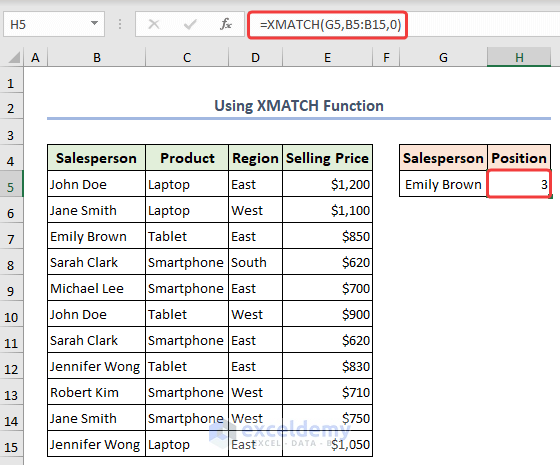
• As a result, we have successfully run the horizontal lookup and got the first 3 region names from the column.

20. Using XMATCH Function

The XMATCH function returns the relative position of a specific value from a dynamic range. In this section, we are using the XMATCH function to search for the position of the row where the Salesperson named Emily Brown exists.

• Select a cell (H5), apply the below formula, and click ENTER.

• As a result, you will get the position of the cell in the worksheet.

Advantages of Dynamic Arrays in Excel

1. With dynamic arrays, you can use regular formulas that automatically handle multiple values without requiring special array syntax.
2. Functions like SORT, FILTER, UNIQUE, and SEQUENCE enable the extraction of data to easily and quickly solve complicated problems.
3. Dynamic arrays provide better error handling by returning an error for one element without affecting the other elements in the worksheet.

Disadvantages of Dynamic Arrays in Excel

1. Dynamic arrays are available in Excel 365, Excel 2021, and newer versions. If you need to share your workbook with users who have older Excel versions, they won’t be able to use dynamic array functions.
2. Dynamic arrays do have some limitations with user-defined functions. Some user-defined functions (custom functions created with VBA) may not work seamlessly with dynamic arrays.

Difference Between Dynamic Arrays and Traditional Arrays in Excel

1. Dynamic array functions use regular formula syntax, just like any other Excel function. On the other hand, traditional array formulas require a special syntax, typically involving array operators. You also need to manually enclose the formula in the desired range using CTRL+SHIFT+ENTER.
2. Excel introduced new dynamic array functions like SORT, FILTER, UNIQUE, and SEQUENCE, which enable powerful data manipulation and analysis. While traditional array formulas can perform similar tasks, they often require more complex formula structures.

Compatibility Issues of Dynamic Arrays in Excel

Compatibility issues arise with dynamic arrays in Excel due to their limited availability in older versions of Excel. After opening the file with an older version of Excel you will find errors just like the following image for dynamic arrays.

What to Do When Dynamic Arrays Formula Is Not Working in Excel

While dynamic arrays in Excel offer numerous advantages, they can also lead to certain errors if not used correctly. Some common errors associated with dynamic arrays are described below.

1. #SPILL! Error

Most of the time you will find #SPILL! Error as it happens when the formula’s output cannot fit into the available space in the adjacent cells.

• Here we choose a cell (G5), write the formula and press ENTER.

• As a result, you will find #SPILL! Error as there are values inserted previously inside the output column.

• Now, selecting cell (G10), click DELETE to remove the content from the cell.

• Finally, you will get the output without #SPILL! Error.

2. #REF! Error

The #REF! error in dynamic arrays occurs when a formula refers to a cell or range that is invalid or unavailable due to changes in the spreadsheet.

• Simply, use the below formula with the exact range to solve the #REF! error problem.

3. #NAME? Error

A #NAME? error occurs when the formula contains a named range and the name range does not exist. Sometimes due to inappropriate references, it might occur too.

• In this part, we select a cell (G5), write the below formula, and hit ENTER.

• Thus we will get #NAME? Error as we used an inappropriate range inside the formula.

• Simply, use the below formula which refers to the exact cell range to solve #NAME? error problem.

Things to Remember

• While using dynamic arrays be cautious about creating circular references with dynamic arrays, as it can lead to incorrect results and a circular reference warning.

Frequently Asked Questions

1. How do I handle errors in dynamic array formulas?

You can use error-handling functions like IFERROR or IFNA to manage potential errors that might occur with dynamic arrays and display meaningful messages or alternative results.

2. Can I use dynamic array functions with traditional array formulas?

It is generally not recommended to combine dynamic array functions with traditional array formulas, as it can lead to conflicts and errors.

3. How do I avoid circular references with dynamic arrays?

Avoid referencing a dynamic array formula’s own spill range or creating formulas that depend on each other in a circular manner to prevent circular reference errors.

Conclusion

Dynamic arrays in Excel offer significant advantages, simplifying formulas, enabling automatic spill ranges, and providing better error handling. However, you have to be mindful of compatibility with older Excel versions. Overall, using dynamic arrays can lead to more efficient and powerful spreadsheet solutions in Excel 365 and newer versions. Take a tour of the practice workbook and download the file to practice by yourself. Please inform us in the comment section about your experience. We, the Exceldemy team, are always responsive to your queries. Stay tuned and keep learning.