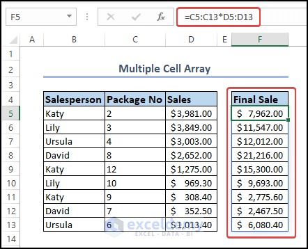
Get the final sale of values by multiplying sales by the number of the packages:
What is Array Formula
An array formula can execute many calculations on one or more items and return many results or only one. There are Multiple Cell array formulas and Single-cell array formulas.
Multiple Cells Array Formula
- Select F5 and enter the following formula:
=C5:C13*D5:D13
- There is an array symbol in F5:F13.

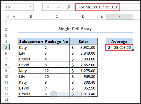
Single Cell Array Formula
To get the output in a single cell, enter the following formula in F5.
=C5:C13*D5:D13
The Summation of the sales is displayed in F5.
Read More: What Is an Array in Excel?
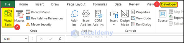
How to Launch the VBA Editor in Excel
Press Alt+F11 or use the Visual Basic command in the Developer tab.
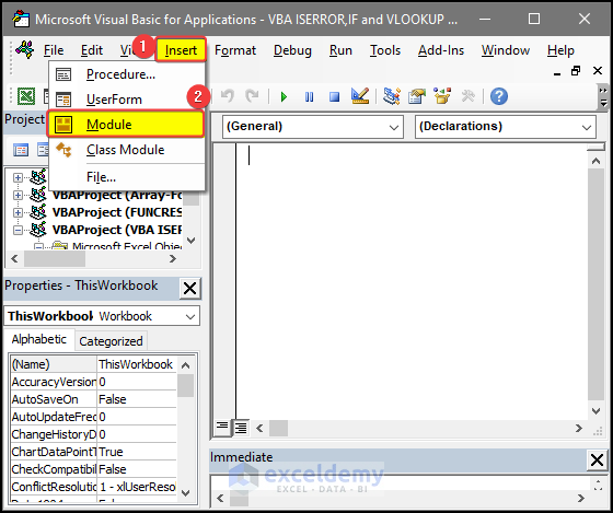
- Select Insert > Module, and you will see the VBA editor to enter the code.
Example 1 – Create a One Dimensional Array Formula with Constant Values in Excel
- Use the names of different products inside inverted commas and separate each product with semicolons. Enclosed the whole list with second brackets.
- Enter the formula in B4:
={"Apple";"Orange";"Kiwi";"Tomato";"Banana"}
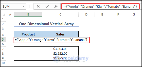
- Press ENTER.
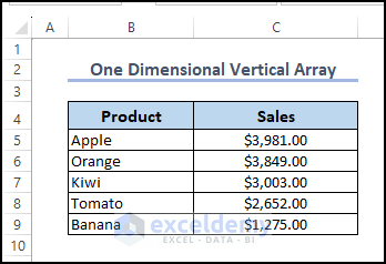
This is the output.
If you want to enter the name of the products horizontally, change the formula.
- Enter the following formula in C4:
={"Apple", "Orange", "Kiwi", "Tomato", "Banana"}
The names of different products were used inside inverted commas and separated with commas. The whole list was enclosed with second brackets.
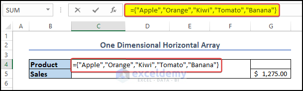
- Press ENTER.
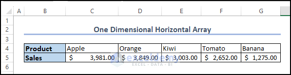
This is the output.
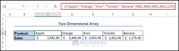
Example 2 – Create a Two Dimensional Array Formula with Constant Values in Excel
- Enter the formula in C3:
={"Apple", "Orange", "Kiwi", "Tomato", "Banana";3981,3849,3003,2652,1275}
The name of the products and the sales values are separated with commas. The final product name is separated by a semicolon from the sales value of the first product.
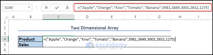
- Press ENTER.
This is the output.
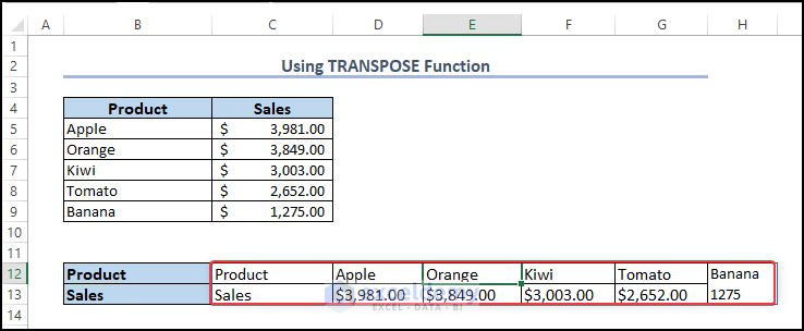
Example 3 – Using the TRANSPOSE Function with an Array Formula to Reverse Rows and Columns
- Enter the formula in C11:
=TRANSPOSE(B4:C9)
B4:C9 is the range of the rows to transform into columns.
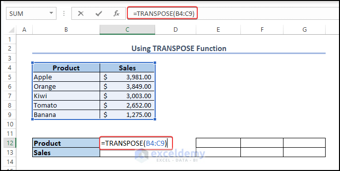
- Press ENTER.
This is the output.
Example 4 – Create an Array Formula with the SUM Function in Excel
- Enter the formula in D10:
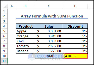
=SUM(C5:C9*D5:D9)
C5:C9 is the sales, and D5:D9 is the discounts.
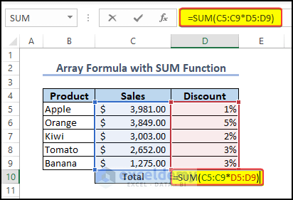
- Press ENTER.
This is the output.
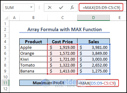
Example 5 – Create Array Formula with the MAX Function in Excel
- Enter the formula in D10:
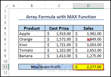
=MAX(D5:D9-C5:C9)
C5:C9 is the Cost Prices, and D5:D9 is the Sales values.
- Press ENTER.
- This is the output.
Example 6 – Create an Array Formula for Multiple Rows in Excel
Calculate the bonus earned by the employees:
- Use the following formula in F4.
=(D4:D8-C4:C8)*E4:E8
C4:C8 is the Cost Prices, D4:D8 is the Sales values, and E4:E8 is the %.
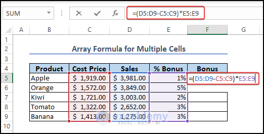
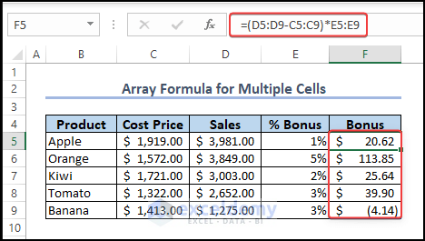
- Press ENTER.
This is the output.
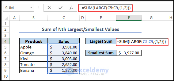
Example 7 – Create an Array by Summing the Nth Largest or Smallest Numbers
- Enter the following formula in E4.
=SUM(LARGE(C4:C8,{1,2}))
C4:C8 is the sales values, and {1,2} extracts the largest two values.
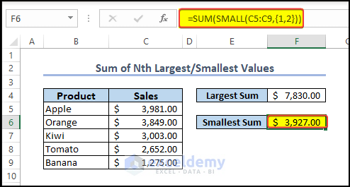
- Enter the following formula in E6 to get the sum of the lowest two sales values.
=SUM(SMALL(C4:C8,{1,2}))
C4:C8 is the sales values, and {1,2} extracts the smallest two values.
Example 8 – Create an Array with Multiple Criteria in a Formula
Count the total number of times the products Mango and Orange were sold by Lily:
=SUM(COUNTIFS(B4:B12,"Lily",C4:C12,{"Mango","Orange"}))
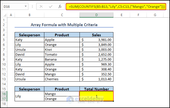
Formula Breakdown
- COUNTIFS(B4:B12,”Lily”,C4:C12,{“Mango”,”Orange”}) → becomes
Output → {0,1}
- SUM(COUNTIFS(B4:B12,”Lily”,C4:C12,{“Mango”,”Orange”})) → becomes
SUM({0,1})
Output → 1
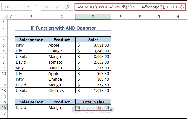
Example 9 – Combine the IF and SUM Functions to Create an Array Formula in Excel
Calculate the total sales value of the product Mango sold by David:
- Enter the formula in D15:
=SUM(IF(((B4:B12="David")*(C4:C12="Mango")),(D4:D12)))
If both conditions B4:B12=”David” and C4:C12=”Mango” are met in a row, the corresponding sales values will be extracted and the values will be added.
- Press ENTER.
This is the output.
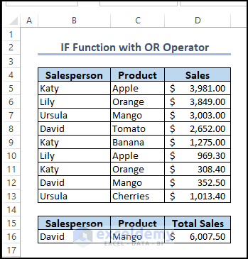
Example 10 – Combine the IF Function and the OR Operator to Create an Array Formula in Excel
Calculate the total sales value of the product Mango sold by David:
- Enter the formula in D15:
=SUM(IF(((B4:B12="David")+(C4:C12="Mango")),(D4:D12)))
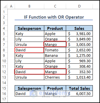
If any of the conditions B4:B12=”David” and C4:C12=”Mango” are met in a row, the corresponding sales values is extracted and the values are added.
- Press ENTER.
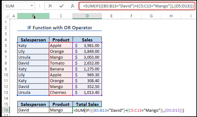
This is the output.
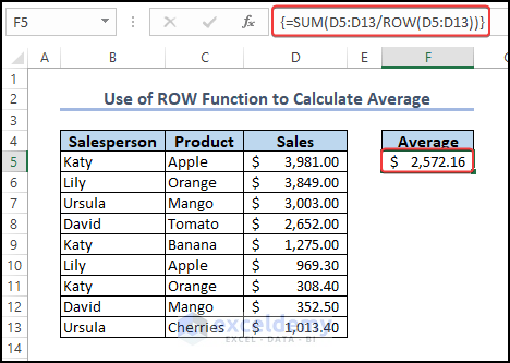
Example 11 – Use the ROW Function to Create an Array Formula in Excel
- Enter the formula in F5:
=SUM(D5:D13/ROW(D5:D13))
- Press ENTER.
This is the output.
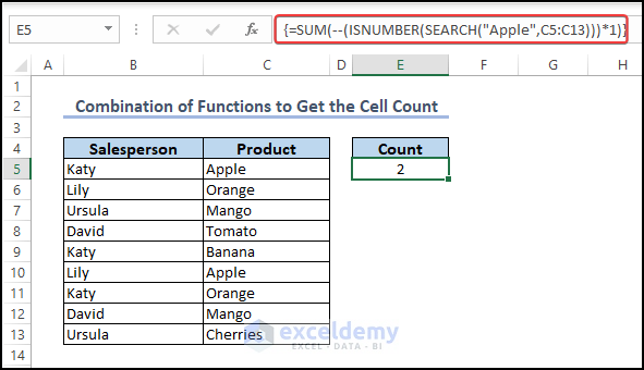
Example 12 – Create an Array Formula to Count Cells in a Range
- Enter the formula in E5:
=SUM(--(ISNUMBER(SEARCH("Apple",C5:C13)))*1)
- Press ENTER.
This is the output.
Example 13 – Create an Array Formula to calculate the Average in a Range
- Enter the formula in F5:
=SUM(D5:D13)/COUNT(D5:D13)
- Press ENTER.
This is the output.
How to Create a Dynamic Array Formula in Excel – 6 Examples
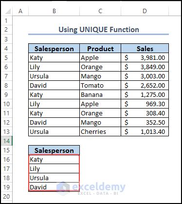
Example 1 – Using the UNIQUE Function to Create an Array Formula in Excel
Extract the unique names in the SalesPerson column:
- Enter the following formula in B15.
=UNIQUE(B4:B12)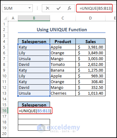
This is the output.
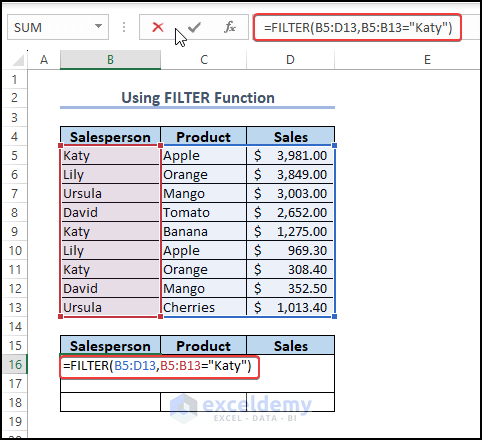
Example 2 – Use the FILTER Function to Create an Array Formula in Excel
Extract the data for Katy:
- Enter the formula in B15:
=FILTER(B5:D13,B5:B13="Katy")B4:D12 is the range, and B4:B12=”Katy” is the criterion for filtering.
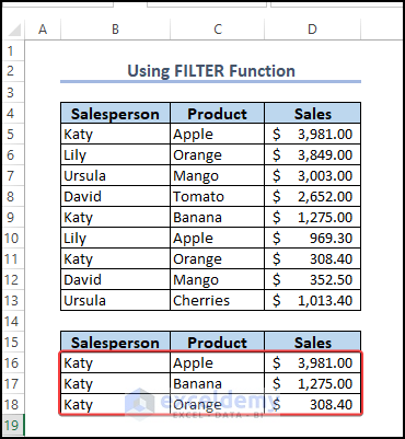
- Press ENTER.
This is the output.
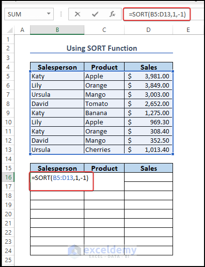
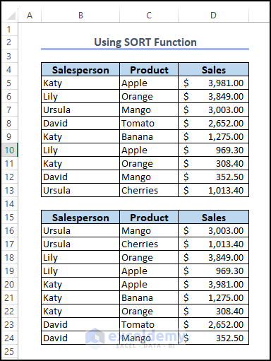
Example 3 – Applying the SORT and the SORTBY Functions to Create an Array Formula in Excel
- Use the following function in B15.
=SORT(B4:D12,1,-1)
B4:D12 is the dataset, 1 is the number of the column to be sorted, and -1 returns a descending order.
- Press ENTER.
This is the output.
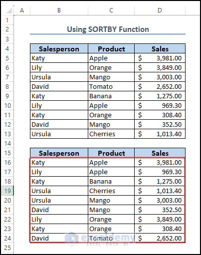
- Use the SORTBY function.
=SORTBY(B4:D12,C4:C12,1)
B4:D12 is the dataset, C4:C12 is the column to be sorted, and 1 returns an ascending order.
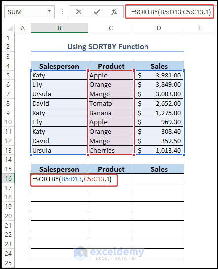
- Click OK.
Salespersons are sorted by Product.
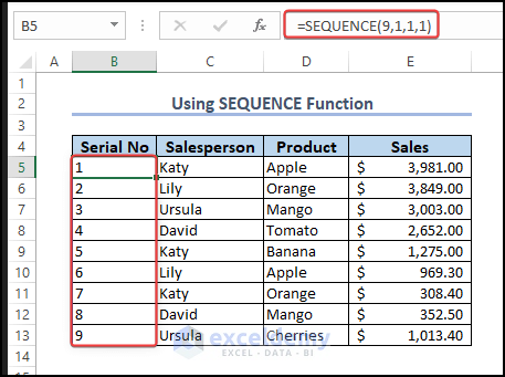
Example 4 – Applying the SEQUENCE Function to Create an Array Formula in Excel
Enter serial numbers from 1 to 9 in a sequence:
- Enter the following formula in B4.
=SEQUENCE(9,1,1,1)
9 is the total rows, 1 is the column number, 1 is the starting number, and 1 is the step number.
Example 5 – Utilizing the RANDARRAY Function to Create an Array Formula in Excel
Create random serial numbers:
- Enter the following formula in B4.
=RANDARRAY(9,1,1,9,TRUE)
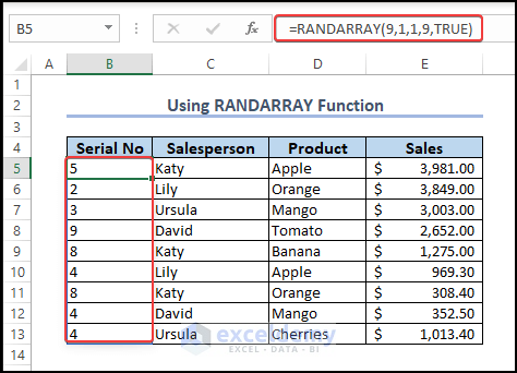
Note:
The serial numbers generated by this function will automatically change if you refresh.
Example 6 – Using the XLOOKUP Function to Create an Array Formula in Excel
- Enter the formula in F5:
=XLOOKUP("Katy",Table1[Salesperson],Table1[Sales],1,0)
- Press ENTER.
This is the output.
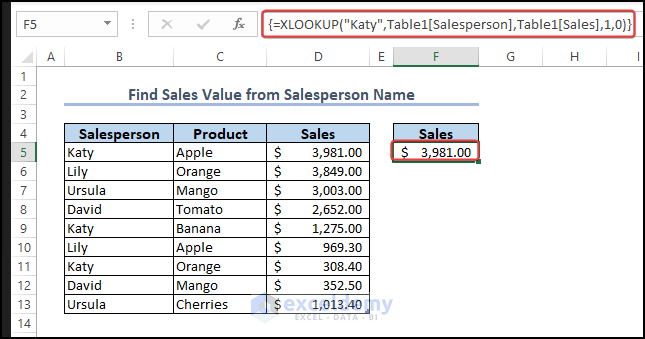
Note:
Convert data to a table before applying this method.
Why is the Array Formula Not Working in Excel?
Common issues:
- Not entering the formula correctly: Press Ctrl+Shift+Enter instead of Enter.
- Incorrectly referencing cells: If you reference a cell that contains a formula, it will not return an array.
- Using incompatible formulas: Not all formulas can be used in array formulas.
- Too much data: Too much data can cause the formula to fail or Excel to crash.
- Calculation mode: Make sure your calculation mode is set to Automatic.
- Conflicting add-ins: Disable add-ins and check if the issue is solved.
Excel Array Constants
There are two types of array constants.
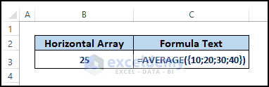
Horizontal Array Constants
- Enter the following formula in the cell and get the maximum of the array values.
=MAX({5,7,2,9})
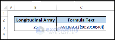
Longitudinal Array Constants
- Enter the following formula to see the longitudinal array average.
=AVERAGE({10;20;30;40})
Limitations of the Array Formulas in Excel
- Limited editing: Once an array formula is entered into a cell, it cannot be edited like a regular formula. You must edit the entire formula.
- Limitations on number of elements: Excel has limitations on the number of elements that can be used in an array formula. The maximum number of elements in an array formula is 1,048,576.
Frequently Asked Questions
What does {} do in Excel?
The curly braces {} are used to enclose an array formula.
How do I create an array list in Excel?
Create a Named range and then create a list.
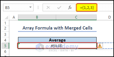
Can Array formulas be entered into a Merged cell?
No. Errors may occur.
Things Need to Remember
- Array formulas can only be entered in a single cell. The result will be displayed in that cell. However, the formula can reference a range of cells.
- The curly braces {} must be entered manually when using the formula.
- Make sure the range of cells referenced in the array formula is the same size and shape as the result you want to return.
Download Practice Workbook
Download the following workbook.
Related Articles
<< Go Back to Array Formula | Excel Formulas | Learn Excel
Get FREE Advanced Excel Exercises with Solutions!
