Introduction to Excel XLOOKUP Function
- Summary:
Searches a range or an array for a match and returns the corresponding item from a second range or array.
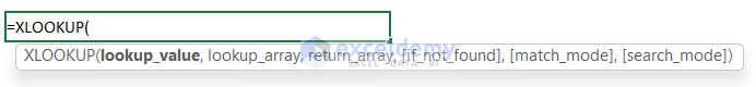
- Syntax:
=XLOOKUP (lookup_value, lookup_array, return_array, [if_not_found], [match_mode], [search_mode])- Arguments:
| Argument | Required/Optional | Explanation |
|---|---|---|
| lookup_value | Required | It’s the specified value that needs to be searched for in the data table. |
| lookup_array | Required | The lookup_array is a range of cells or an array where the lookup_value will be searched for. |
| return_array | Required | It’s the second range of cells or an array from where the output data will be extracted. |
| if_not_found | Optional | If the lookup value is not found, a customized message can be inserted using this argument in text format. |
| match_mode | Optional | It defines if the function will look for an exact match based on specified criteria or a wildcard character match. |
| search_mode | Optional | It denotes the search order (in ascending or descending order, from last to first or first to last). |
- Return Parameter:
The XLOOKUP function allows you to look for a value in a dataset and return the corresponding value in some other row/column.
How to Use XLOOKUP Function in Excel: 11 Practical Examples
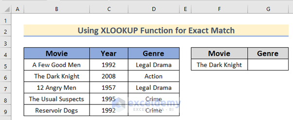
Example 1 – Use the XLOOKUP Function for Exact Match
We will provide the movie name and derive the genre using the XLOOKUP function.
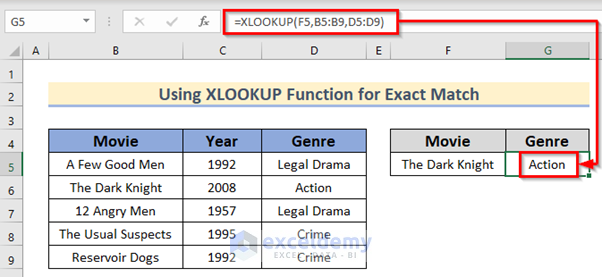
Steps:
- Select Cell G5 and insert the following formula.
=XLOOKUP(F5,B5:B9,D5:D9)- Press Enter to get the lookup value.
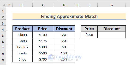
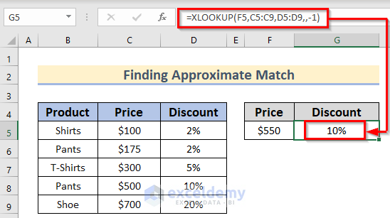
Example 2 – Find an Approximate Match Using the Excel XLOOKUP Function
We will find the discount for the given price.
Steps:
- Enter the following formula in Cell G5.
=XLOOKUP(F5,C5:C9,D5:D9,,-1)- Press Enter to find the corresponding value of Discount.
- The approximate matches can be done by another approach.
- Enter the following formula in Cell G5.
=XLOOKUP(F5,C5:C9,D5:D9,,1)- Press Enter.

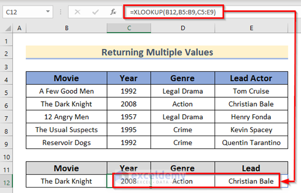
Example 3 – Return Multiple Values by Applying the XLOOKUP Function in Excel
We will find all the listed details for a given movie name.
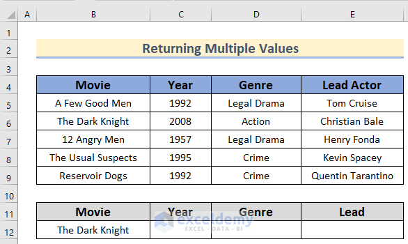
Steps:
- Select Cell C12 and insert the following formula.
=XLOOKUP(B12,B5:B9,C5:E9)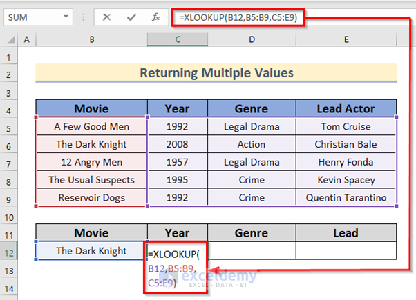
- Press Enter to get all the details available of that movie.
Read More: How to Use XLOOKUP to Return Blank Instead of 0
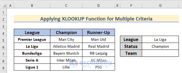
Example 4 – Apply the Excel XLOOKUP Function for Multiple Criteria
We have selected a sample dataset of the roll of honor of 5 European leagues. Now, we will set the name of the league and the status as criteria and look for the corresponding Team.
Steps:
- Enter the following formula in Cell G7.
=XLOOKUP(G6,C4:D4,XLOOKUP(G5,B5:B9,C5:D9))- Press Enter.
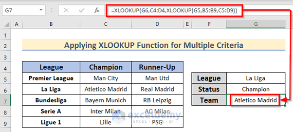
How Does the Formula Work?
- We have used two XLOOKUP. Within the first XLOOKUP, we checked the status of the team.
- We have set the second XLOOKUP at the return_array
- Within this second XLOOKUP function, we have checked the league name and set the team names as the return_array.
- We have found the name of the team.
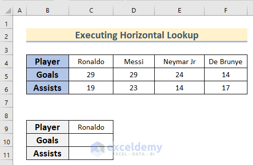
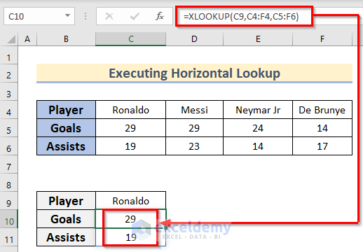
Example 5 – Execute Horizontal Lookup Using XLOOKUP Function
The sample dataset below contains several players with their goals and assists. We will find the goals and assists for a given player. The name of the player will be our lookup_value and stored in Cell C9.
Steps:
- Enter the following formula in Cell C10.
=XLOOKUP(C9,C4:F4,C5:F6)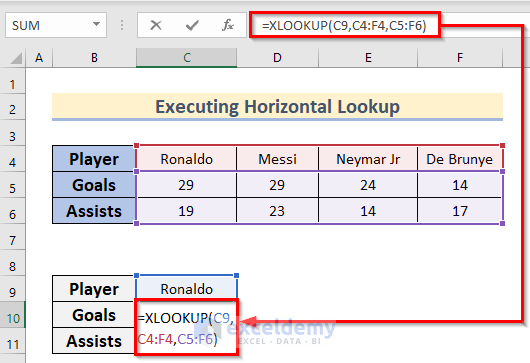
- Press Enter.
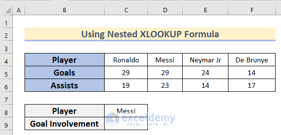
Example 6 – Use Nested XLOOKUP Formula in Excel
From the scorer dataset, we want to find the goal involvement (sum of goals and assists) for a given player.
Steps:
- Select Cell C9 and insert the following formula.
=SUM(XLOOKUP(C8,C4:F4,C5:F5),XLOOKUP(C8,C4:F4,C6:F6))- Press Enter.
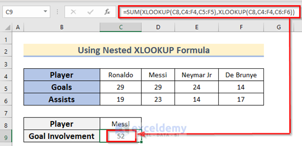
How Does the Formula Work?
- The two XLOOKUP functions will provide goals and assists respectively for a player.
- The SUM function will add them together and provide the result.
Example 7 – Solve #N/A Error Using XLOOKUP Function in Excel
From our movie dataset if we set a value that is within our table and find the value. If we set a movie name that is not on the table, then the #N/A error occurs.
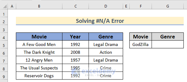
We provided Godzilla as the movie name and the error occurred.
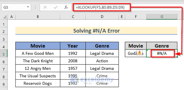
To remove the error, follow the steps given below.
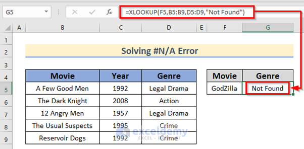
Steps:
- Enter the following formula in Cell G5.
=XLOOKUP(F5,B5:B9,D5:D9,"Not Found")- Press Enter to execute the formula.
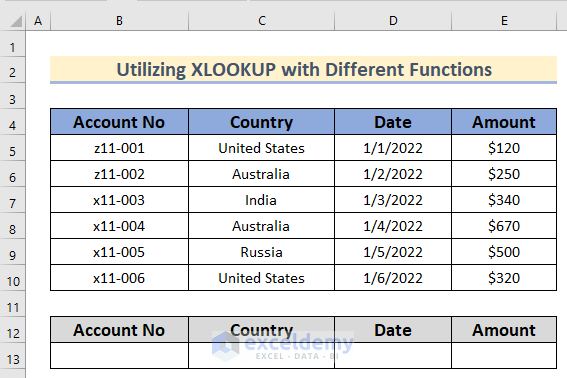
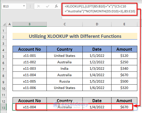
Example 8 – Utilize XLOOKUP with Different Functions for Complex Criteria
We have a sample dataset containing some bank Account No, their corresponding Country, the amount of cash and the Date of transaction of those accounts.
Search the data for the account that begins with “x” and Country is “Australia” and the month is not March.
Steps:
- Select Cell B13 and insert the following formula.
=XLOOKUP(1,(LEFT(B5:B10)="x")*(C5:C10="Australia")*NOT(MONTH(D5:D10)=3),B5:E10)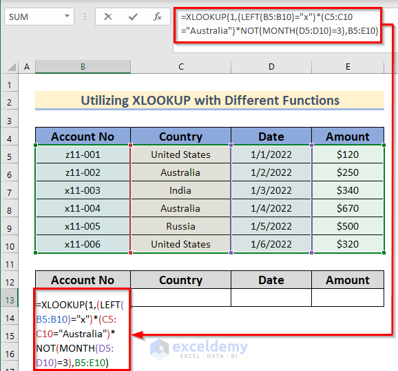
- Press Enter.
How Does the Formula Work?
- The LEFT function will check if there is “x” on the left of the given cell range B5:B10.
- The MONTH function will find out the month value of the cell range D5:D10.
- The NOT function will check if the resultant of the MONTH is not equal to 3.
- Using the results of these functions, the XLOOKUP will return the desired data range.
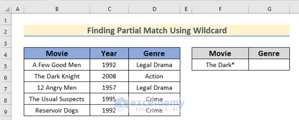
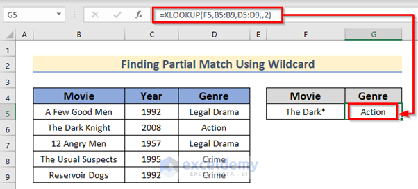
Example 9 – Apply Excel XLOOKUP Function to Find Partial Match Using Wildcard
In the movie sample dataset, we will find the genre of a given movie with a wildcard.
Steps:
- Enter the formula given below in Cell G5.
=XLOOKUP(F5,B5:B9,D5:D9,,2)- Press Enter.
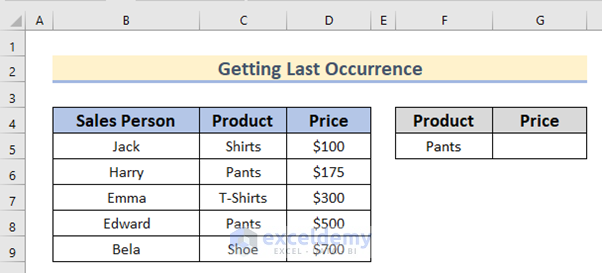
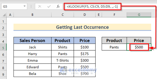
Example 10 – Get the Last Occurrence Using XLOOKUP in Reverse Order
In our sample dataset below, Pants are sold 2 times. We want to find out the price of the pants in the last occurrence.
Steps:
- Insert the following formula in Cell G5.
=XLOOKUP(F5, C5:C9, D5:D9, ,,-1)- Press Enter to find the Price of the pants in the last occurrence.
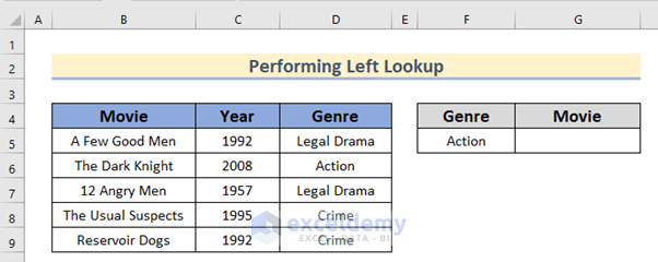
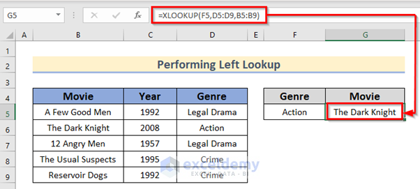
Example 11 – Perform Left Lookup Applying Excel XLOOKUP Function
Find a movie name using Action as Genre.
Steps:
- Insert the formula given below in Cell G5.
=XLOOKUP(F5,D5:D9,B5:B9)- Press Enter.
Things to Remember
- You can also insert or type the lookup_value directly within the XLOOKUP function.
Download Practice Workbook
<< Go Back to Excel Functions | Learn Excel
Get FREE Advanced Excel Exercises with Solutions!

Excellent and Helpful
Hello Ravam,
Thanks for your feedback and appreciation. Glad to hear that it was helpful.
Keep exploring Excel with ExcelDemy!
Regards,
ExcelDemy