What Is an Array in Excel? (5 Ideal Uses)

Today, I will talk about the basics of Excel Array Formulas. Most Excel users find it one of Excel’s most challenging topics to understand. There are several articles online already on this topic.

Then why am I writing this one again?

I found most of those articles are complex for beginners. I will write a series of articles on Array Formula (this is the first one) and make understanding Excel Array Formulas as easy as possible.

Those who want to become a master in Excel formulas must have to know how to handle arrays in formulas. Before understanding array formulas, you have to know what Excel Arrays are. If you know any programming language, then you know arrays well. If you have no idea about a programming language, then don’t worry. It is straightforward.

Introduction to Array in Excel

An Array is just a list of some items. The items might be some values like this list (green colored in the following image), some text like this list (red-colored in the following image), or mixed up with both values and text like this list (blue colored in the following image).

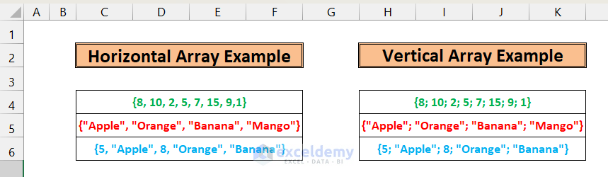
There is something common between these three lists. All of the items are listed within curly braces{ }. And another thing is when the items are text, they are listed within double quotation marks ( ” “ ). The first array has a total of 8 items. The second array has a total of 4 items, and the last array has a total of 5 items.

There are the same arrays on the right side of the worksheet (above image), but the items are separated by semicolons ( ; ). The difference between commas and semicolons is that comma-separated arrays are entered into the worksheet horizontally, and semi-colon-separated arrays are entered vertically. An array can also have both commas and semicolons, called a multi-dimensional array. In this article, I shall not cover the multi-dimensional array concept. It will be covered in detail later.

5 Different Examples to Use Array in Excel

In this section, I will demonstrate 5 essential examples to use Array in Excel which will help you to learn all the basic aspects of excel array.

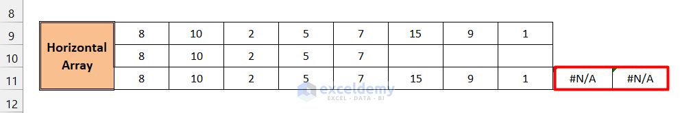
1. Enter a Horizontal Array Formula in Excel

Let’s see how you can input an array into a cell or more than one cell. Follow the steps below:

• The first array has 8 values, so you need to select 8 cells before entering this array into the worksheet.
• First, select a total of 8 cells horizontally (from cell C9 to J9).
• Now on the formula bar, type the followings:

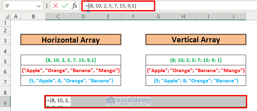
• Now press CTRL+SHIFT+ENTER ( Unlike regular formulas where we only press ENTER button for entering, here we have to press CTRL+SHIFT+ENTER, which is a major difference between array formula and regular formula)
• Consequently, you will find that the array values are filled in the eight selected cells (horizontally).

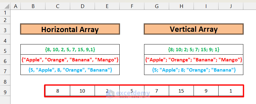
• Let’s now see what happens when we enter the same array in less than eight cells. I select five horizontal cells this time (from cell C10 to G10), type the same array formula, and press CTRL+SHIFT+ ENTER keys on the keyboard. You see the first 5 values of the array have entered into the selected 5 cells. On the other hand, the remaining 3 values are not entered.

• Let’s now check what happens when we select more than 8 cells to enter this array. I select 10 cells horizontally (from cell C11 to L11), type the same array, and press CTRL SHIFT and ENTER keys on the keyboard. You see, the first 8 cells are filled with the 8 values, and the rest 2 cells are showing errors.

2. Insert a Vertical Array Formula in Excel

Let’s now see how we can enter a vertical array. To do that, follow the steps below:

Steps:

• Select any vertical 8 cells. Here we select G3:G10
• Now in the formula bar, write the following.

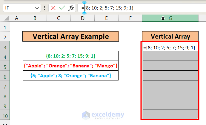
• Now press the CTRL+SHIFT+ENTER keys on the keyboard.

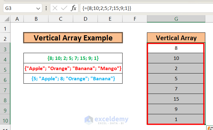
• So this is how you can enter a vertical array.

3. Introduce Range with Repetitive Array in Excel

Now that we have learned how to enter horizontal and vertical arrays, we will now focus on how we can enter an array multiple times in a selected range of cells. To do that, follow the steps below.

Steps:

• First, select a range that has 5 cells horizontally, and 8 cells vertically (from cell I3 to M10),
• Now in the formula bar, again type the array values.

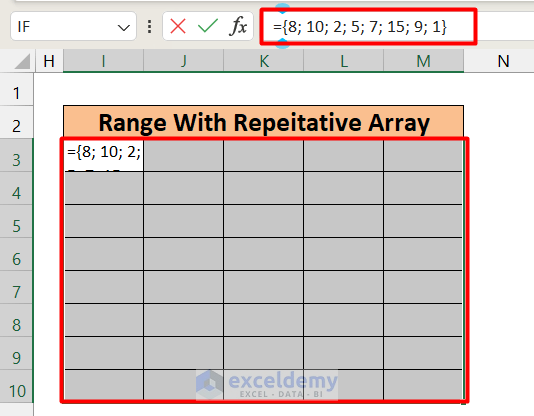
• After that, press the CTRL+SHIFT+ ENTER keys on the keyboard.
• You see, the range is filled with the repeated array.

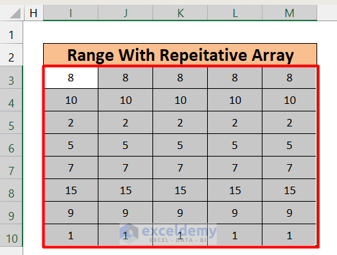
• So this is how we can enter an array multiple times.

4. Analyze an Array Formula in Excel

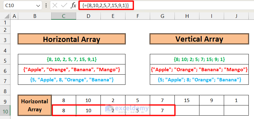
• Until now, we have entered arrays in excel. But now we will look at how Excel stores an array.
• Take a look at the formula bar. You should see a new curly brace added before the equal sign.

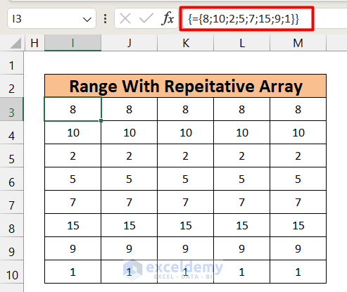
• We have entered only the equal sign and the curly bracket with the values. After pressing CTRL SHIFT and ENTER keys on the keyboard, a new curly brace is enclosing all the contents in the formula bar.
• When you get this type of formula structure, you will treat it as an Array formula. This sign differentiates the array formula from a regular Excel formula.

5. Change Array Formula in Excel

You must remember that whatever cell you select within an array formula, the formula is the same for all the cells in the formula bar. So if you want to change the array formula, you can do it by modifying any cell formula you like. For example, C3 and C6 have the same cell formula in the array below.

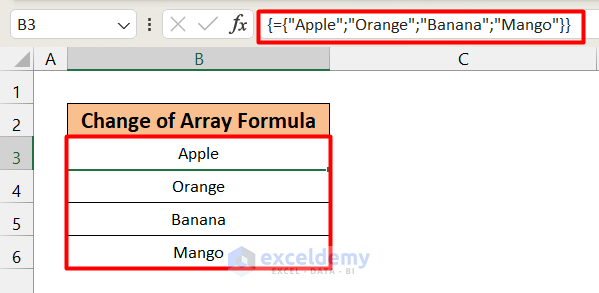
Let’s say we want to modify the array formula: we will replace the Orange with Watermelon. We can do that in the following way:

• Select any random cell of the array. Here we have selected B6.

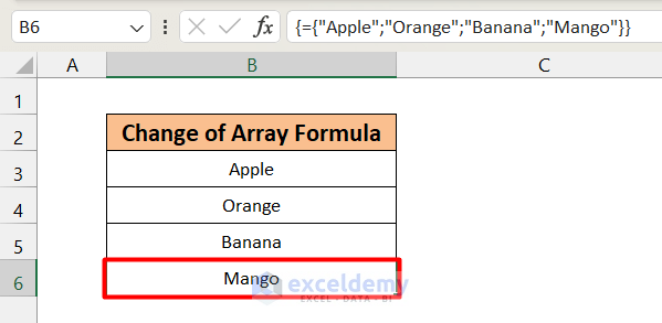
• Now in the formula bar, write the following formula:

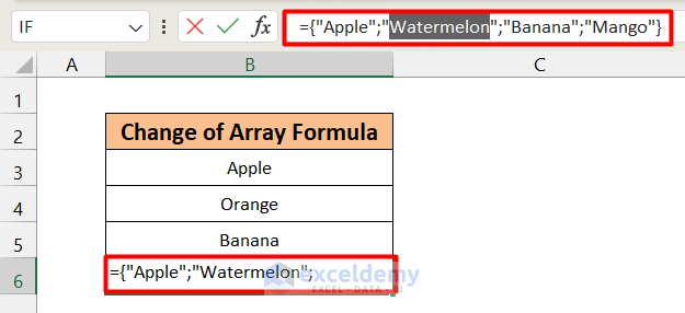
Here we have just written Watermelon in place of Orange, and all the other things are the same.

• Now click CTRL+SHIFT+ ENTER. You will see the following results.

So this is how we can modify an array formula

Note:

• Here, if you press ENTER instead of CTRL+SHIFT+ ENTER, you will get an error message like this.

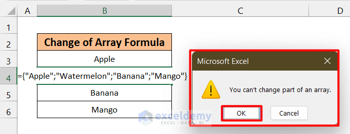
• If you commit the mistake, click OK on the pop-up Dialogue box and again press CTRL+SHIFT+ ENTER. You will get the desired answer.

Quick Summary of Array in Excel

⇒ Example of Arrays in Excel:

1. Horizontal Array (separated by comma): {8, 10, 2, 5, 7, 15, 9, 1}
2. Horizontal Array (separated by comma): {“Apple”, “Orange”, “Banana”, “Mango”}
3. Vertical Array (separated by semicolon): {8; 10; 2; 5; 7; 15; 9; 1}
4. Vertical Array (separated by semicolon): {“Apple”; “Orange”; “Banana”; “Mango”}

⇒ To enter an array formula, you have to use CTRL + SHIFT + ENTER keys simultaneously. I say this keyword combination as CSE.

⇒ For example, an Excel array has 8 elements.

1. You have selected 8 cells to enter that array. Then all the elements will be entered into the cells.
2. You have selected less than 8 cells (say it is 5) to enter that array. Then 5 cells will take the first 5 elements of the array.
3. You have selected more than 8 cells (say it is 12) to enter that array. Then all the 8 elements of that array will be entered into the first 8 cells, and the rest 4 cells will show #N/A error.

⇒ To Edit an array formula: Just select any cell that holds the array → edit the array → and press CTRL + SHIFT + ENTER keys simultaneously. You are done. All the arrays will be edited.

Download Practice Workbook

Download the working files from the link below.

Conclusion

If you find this article helpful, please share this with your friends. Moreover, do let us know if you have any further queries.

Related Articles

• How to Create Array Formula in Excel
• 5 Examples of Using Array Formula in Excel
• How to Copy Array Formula in Excel