COUNTIFS to Count Across Multiple Columns in Excel

COUNTIFS function provides plenty of opportunities to count cells under different criteria across multiple columns or rows. In this article, I’ll try to illustrate with a relatable dataset how we can utilize the COUNTIFS function precisely to count cells across multiple columns under a number of suitable criteria.

Download Practice Workbook

You can download the Excel Workbook that we’ve used to prepare this article. You can modify the values & see new outputs with embedded formulas.

Introduction to COUNTIF

Before getting down to the uses of COUNTIFS, let’s have a look at how the COUNTIF function works since COUNTIFS is a subcategory of the COUNTIF function. The fundamental difference between these two functions is COUNTIFS simply works under more than one criterion while COUNTIF returns values based on a single criterion only.

• Formula Syntax:

COUNTIF(range, criteria)

• Arguments:

range- Range of cells to be selected 

criteria- Criteria of the cells that need to be assigned

• Function:

Counts the number of cells within the range that meet the given condition.

• Example:

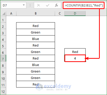
In the picture below, a list of color names is given. If we want to know how many times Red is there then we have to type in the output cell-

After pressing Enter, we’ll see there are 4 instances of Red in the list.

1. Using COUNTIFS to Count Cells across Multiple Columns Under Different AND Criteria

Our dataset consists of the sales profits of several brand computers. In our first criteria, we’ll determine how many HP desktops have been sold with more than $100 profit.

📌 Steps:

➤ In Cell F16 for our dataset, we have to type-

➤ Now press Enter & you’ll see a total of 2 counts of HP desktops with more than $100 profits.

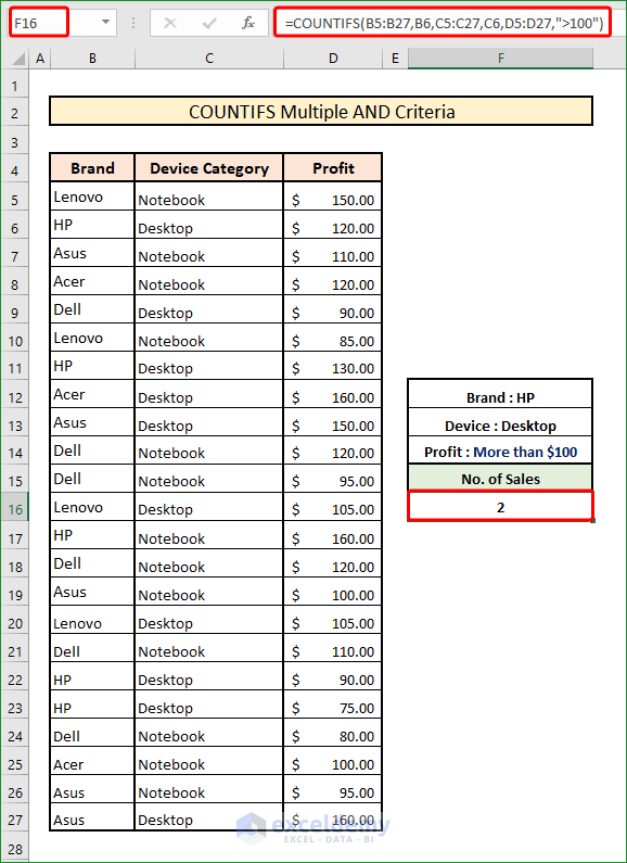
When we’re adding multiple criteria in the COUNTIFS function, we have to use a Comma(,) between two criteria inside the function.

Read more: COUNTIF with Multiple Criteria in Different Columns in Excel

2. Using COUNTIFS to Count Cells across Separate Columns Under Single Criteria

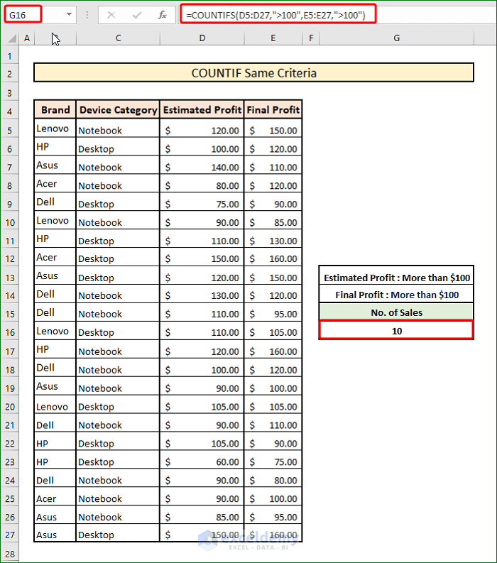
Now in this section, we’ll execute the formula with similar criteria but in different columns. In Columns D & E, Estimated & Final Profits are recorded respectively. We’re going to find the number of cases Estimated & Final profits both have more than $100.

📌 Steps:

➤ In Cell G16, type-

➤ Press Enter & you’ll see a total of 10 findings for our criteria.

Read more: COUNTIFS to Count Across Multiple Columns in Excel

3. Using COUNTIFS to Count Cells across Distinct Columns Under Different OR Criteria

We’ll determine now how many HP desktops, as well as Lenovo Notebooks, have been sold. It means our formula will now incorporate multiple criteria from multiple columns with OR logic.

📌 Steps:

➤ The formula for this criterion in Cell F17 will be-

➤ After pressing Enter, the resultant value will be 6. So there are 6 instances of HP desktops & Lenovo notebooks in our dataset.

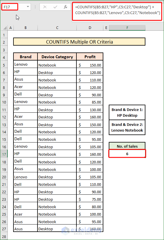
While working with multiple OR criteria, we have to add two different criteria with a Plus(+) between two different COUNTIFS functions.

Read more: COUNTIFS with Multiple Criteria

4. Combining SUM & COUNTIFS to Count Cells across Multiple Columns from Array

While working with both AND & OR criteria, we have to use the SUM function outside the COUNTIFS function as here the COUNTIFS function will return will multiple results that need to be added up. We’ll find out how many HP or Lenovo desktops have more than $100 profits.

📌 Steps:

➤ In Cell F16, we have to type-

➤ Now press Enter & the function will return as 4.

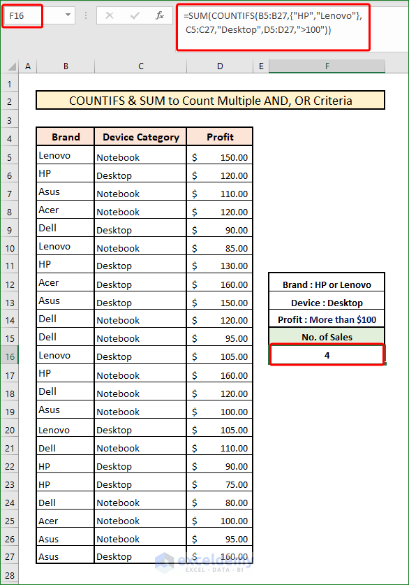
🔎 How Does This Formula Work?

➤ COUNTIFS function returns with the values in an array & the values are- {2,2}

➤ SUM function then simply sums these values up to 4(2+2).

Similar Readings:

• Count Unique Values with Criteria by SUMPRODUCT in Excel
• COUNTIF Multiple Ranges Same Criteria in Excel
• COUNTIF between Two Cell Values in Excel (5 Examples)

5. Incorporating COUNTIFS with Wildcard Characters to Count Cells across Different Columns

In this section, our dataset is not complete. A number of entries are missing. We’ll find out the number of complete entries here.

📌 Steps:

➤ In Cell F16, type-

➤ Press Enter & you’ll find a total of 10 complete entries through this function.

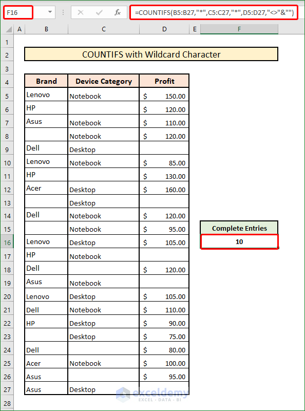
We’re using a Wildcard character here & that is Asterisk(*). It is used to find text strings in a range of cells. We have to put it within Double-Quotes inside the function.

6. Counting Cells with COUNTIFS Function under Dates Condition  across Distinct Columns

With COUNTIFS function, we can also deal with a date input. For our dataset, we’ll now find how many notebooks have been purchased in June, 2021.

📌 Steps:

➤ In Cell F16, we have to type-

➤ Press Enter & the resultant will be 10.

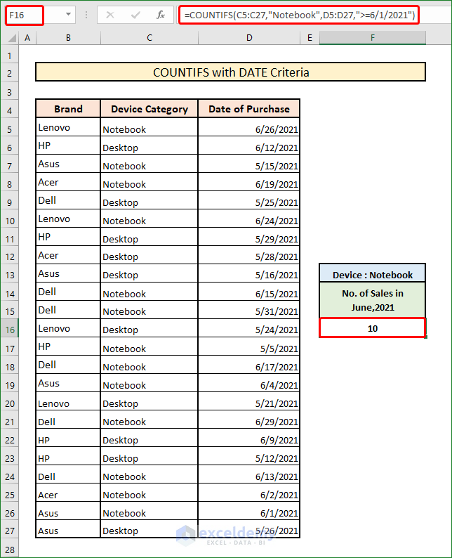
While inputting a date inside a function, we have to maintain the format as MM/DD/YYYY. With Greater or Less Than symbols you can easily insert the logic for date criteria.

7. Using COUNTIFS along with Current Date Functions to Count Cells across Multiple Columns

We can also insert TODAY function while working with COUNTIFS formula. By using TODAY function we can determine preceding or following events to count from the current date. So, for our dataset below, we’ll find out how many devices have been purchased in June & how many of them are yet to deliver from the current date (While preparing this section for the article, the current date was 7/7/2021).

📌 Steps:

➤ In Cell G16, the formula for our criteria will be-

➤ Press Enter & you’ll notice a total of 7 deliveries that are left.

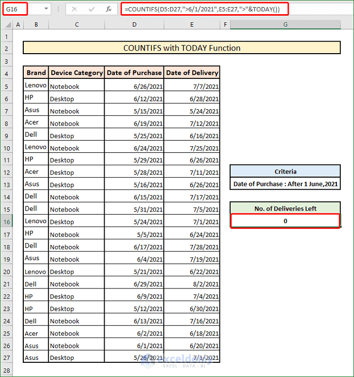
While using TODAY function inside the COUNTIFS formula, we have to add it with conditions by using Ampersand(&) between them.

Concluding Words

I hope, the above uses of COUNTIFS function under multiple criteria across different columns will help you to apply with ease in your regular works with MS Excel. If you think I’ve missed a point or anything to add in this article then please let me know in the comment section. You can also have a look at our other useful articles related to Excel functions on this website.

Related Articles You May Find Interesting

• How to Use COUNTIF to Count Cells Greater Than 0
• Multiple Criteria in Excel Using INDEX, MATCH, and COUNTIF Function
• How to Count the Number of Occurrences in a Date Range in Excel