Sometimes we need to identify the ages of our stock products. Excel has several functions by which we can estimate the age of our stocks. In this context, we will demonstrate to you two different examples of how to use the stock ageing analysis formula in Excel. If you are interested to know, download our practice workbook and follow us.
What Is Stock Ageing Analysis?
The Stock Ageing Analysis is a report usually produced for warehouses, chemical labs, and large departmental stores to check the shelf lives of their inventories or stocks. This report provides us with several advantages in running our business smoothly. The main advantages of making this report are:
- Compare the performance of any type of product of different companies against the benchmarks.
- Identify the slow project and use additional manpower to complete it.
- Track the slowing selling items.
- Sell old products early and if it is not possible, provide the necessary discount offer to consumers.
- Improving decision-making on the accurate time.
- The right amount of inventory production or purchases.
How to Use Stock Ageing Analysis Formula in Excel: 2 Easy Ways
To demonstrate the methods, we are considering a dataset of 15 items. Their arrival dates are in column B. We will calculate their age on the basis of their expiration date. Before that in the Criteria sheet, we will set down our criteria. In this sheet, we define four different categories in four distinct periods. Set the name range of the range of cells B3:C6 as Criteria.

💬 Things You Should Know
We will use the TODAY function in our calculation. The function is a dynamic function. Every day the value of this function will change. So, when you practice using this workbook, the images may not match the images. Don’t get panic. Just follow the steps, and you will get your desired result, at your desired location.
1. Combination of VLOOKUP and TODAY Functions
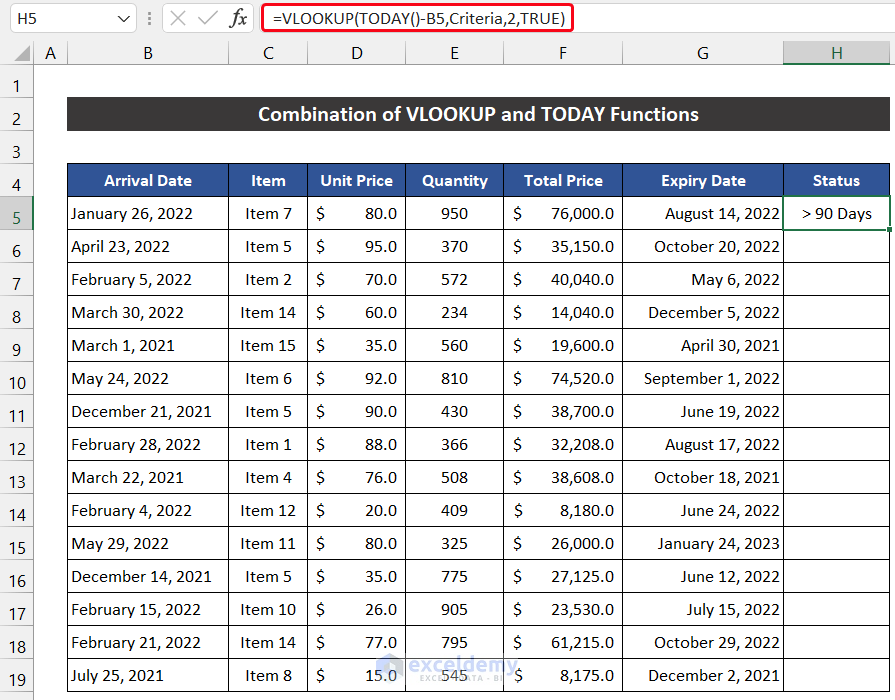
In the example, we are going to use the VLOOKUP and TODAY functions to estimate their ages. Their arrival dates are in column B, item names are in column C, their Unit price is in column D, and Quantity is in column E. Besides that, their Total Price is in column F, and the Expiration Date column is in G. We will show the use of the Stock Ageing Analysis formula in column H based on our criteria.

The steps of this process are given as follows:
📌 Steps:
- First of all, select cell H5.
- Now, write down the following formula in the cell.
=VLOOKUP(TODAY()-B5,Criteria,2,TRUE)
- Press Enter.
- Then, double-click on the Fill Handle icon to copy the formula up to cell H19.
- You will see for all cases the formula will show the age of our stocks.
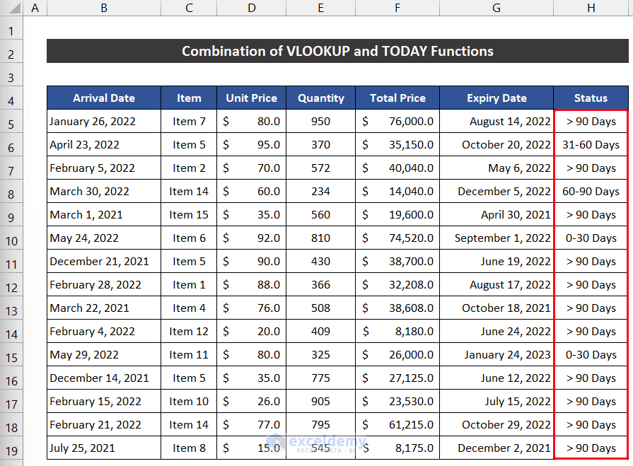
Thus, we can say that our formula worked perfectly and we are able to use the Stock Ageing Analysis formula in Excel.
🔍 Breakdown of the Formula
We are breaking down our formula for cell H5.
👉 TODAY(): This function returns 6/13/2022.
👉 VLOOKUP(TODAY()-B5,Criteria,2,TRUE): The formula returns > 90 Days.
2. Combining VLOOKUP with IF Function
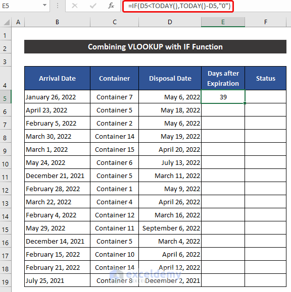
Here, we will use the IF and VLOOKUP functions to evaluate the ages of our items. The arrival dates are in column B, container names are in column C, and their disposal dates are in column D. We will show the ways to use the Stock Ageing Analysis formula to their ages.

The steps to complete this procedure are given below:
📌 Steps:
- First, select cells E4 and F4 and entitle them as Days after Expiration and Status.

- Then, select cell E5 and write down the following formula for the cell.
=IF(D5<TODAY(),TODAY()-D5,"0")
- Press Enter.
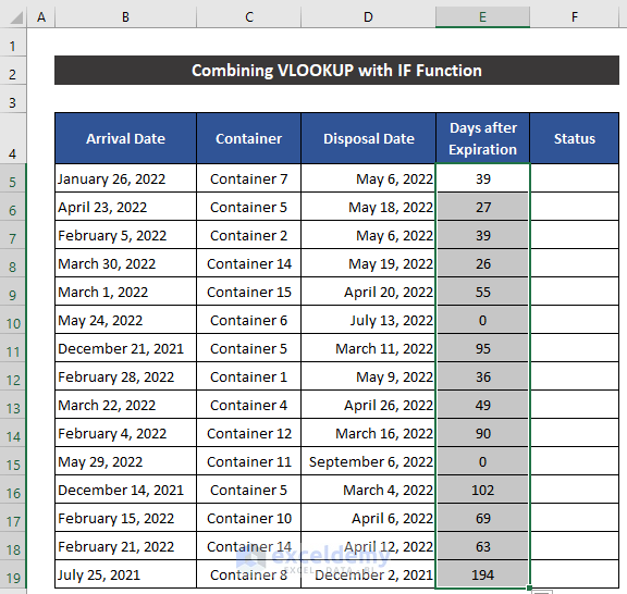
- Now, double-click on the Fill Handle icon to copy the formula up to cell E19.
- After that, in cell F5, write down the following formula to get the Stock Ageing values.
=IF(E5<>0,VLOOKUP(E5,Criteria,2,TRUE)," ")
- Press Enter.
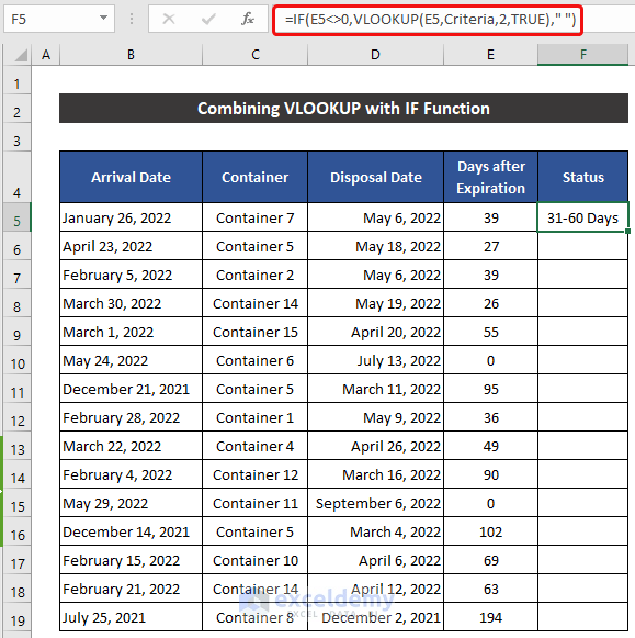
- Now, if you double-click on the Fill Handle icon to copy the formula up to cell F19, you will see you have all the values except for cells F10 and F15. There is an #N/A error.

- The corresponding values of column E of these cells are 0.
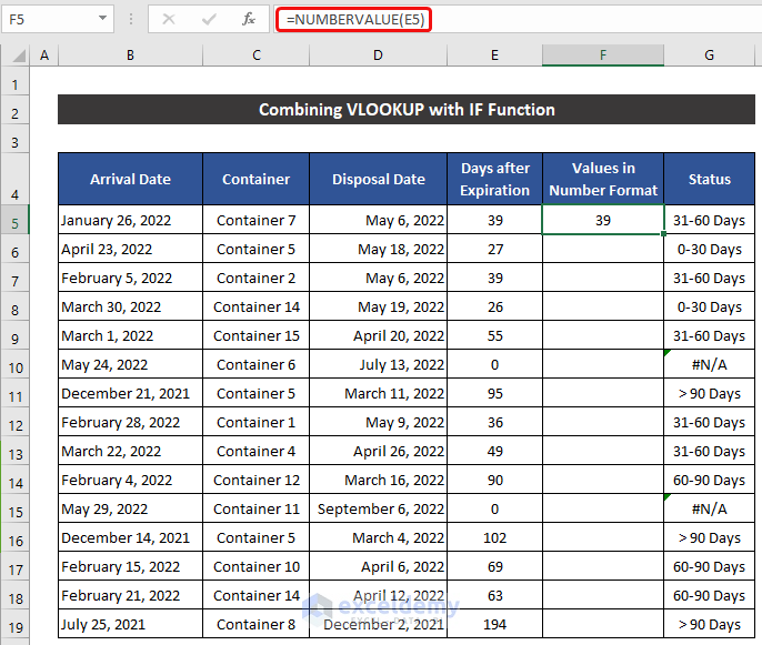
- To avoid this issue, insert a column between columns E and F and title it according to your desire.

- Then, write down the following formula in cell F5.
=NUMBERVALUE(E5)
- Press the Enter key.
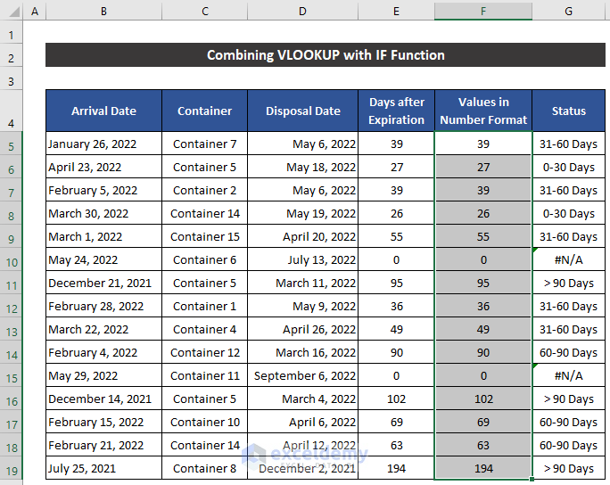
- Similarly, double-click on the Fill Handle icon to copy the formula up to cell F19.
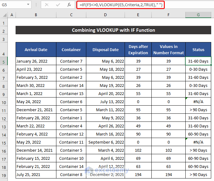
- Now, select cell G5 and modify the logical_test cell reference E5 to F5.
=IF(F5<>0,VLOOKUP(E5,Criteria,2,TRUE)," ")
- Then, press Enter.
- Finally, double-click on the Fill Handle icon to modify all the formulas for every case.
- At last, you will see for all cases the formula will show the age of our stocks.

So, we can say that our approach worked successfully and we are able to use the Stock Ageing Analysis formula in Excel.
🔍 Breakdown of the Formula
We are breaking down our formula for cells E5 and G5.
The formula breakdown for cell E5.
👉 TODAY() : This function returns 6/13/2022.
👉 IF(D5<TODAY(),TODAY()-D5,”0″): This functions returns 38.
Similarly, for cell G5:
👉 VLOOKUP(E5,Criteria,2,TRUE): The formula returns 31-60 Days.
👉 IF(F5<>0,VLOOKUP(E5,Criteria,2,TRUE),” “): The formula returns 31-60 Days.
Download Practice Workbook
Download this practice workbook for practice while you are reading this article.
Conclusion
That’s the end of this article. I hope that this article will be helpful for you and you will be able to use the stock ageing analysis formula in Excel. Please share any further queries or recommendations with us in the comments section below if you have any further questions or recommendations.
<< Go Back to Ageing | Formula List | Learn Excel
Get FREE Advanced Excel Exercises with Solutions!
