
Marketing teams generate huge amounts of data every day, and it can quickly become difficult to manage. A single worksheet may contain campaign names, advertising channels, impressions, clicks, leads, spending, and revenue. You don’t need to be a data analyst to make sense of it, but you do need the right Excel functions in your toolkit.
In this tutorial, we will cover five Excel functions that every marketer should know. These functions can help you summarize, categorize, measure campaign performance, and retrieve information from large datasets.
1. Use XLOOKUP to Retrieve Campaign Information
Marketing workbooks often store campaign targets, budgets, managers, or product information in separate sheets. The XLOOKUP function searches for an item and returns related information from another column.
Basic Syntax:
=XLOOKUP(lookup_value,lookup_array,return_array,[if_not_found])
Unlike VLOOKUP, XLOOKUP can search in either direction and does not require a column number.
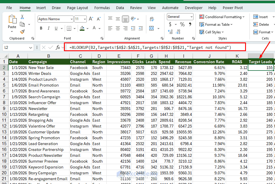
- Extract Target Leads from the Target sheet:
=XLOOKUP(B2,Targets!$P$2:$P$13,Targets!$Q$2:$Q$13,"Target not found")
This formula takes the campaign name from B2 and searches for it in the Campaign column on the Targets worksheet. It returns the corresponding value from the Target Leads column.
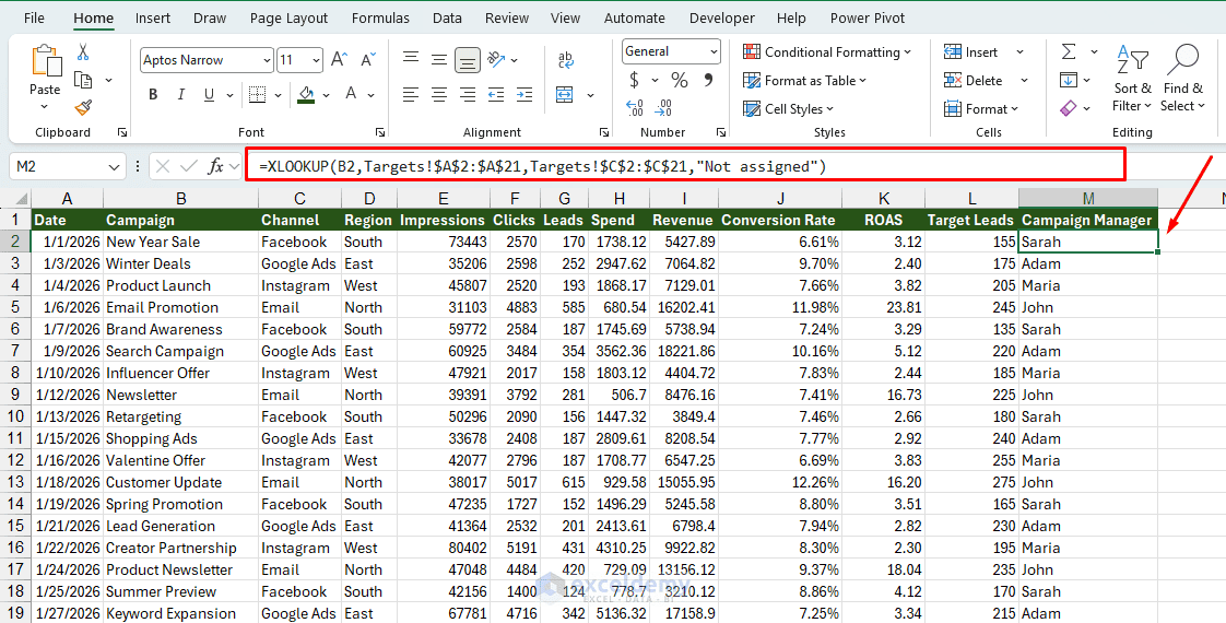
Retrieve the Campaign Manager:
=XLOOKUP(B2,Targets!$P$2:$P$13,Targets!$R$2:$R$13,"Not assigned")
This formula returns the manager responsible for each campaign.
XLOOKUP is particularly useful when campaign details are maintained in a separate master list. Note that XLOOKUP is available in Microsoft 365 and newer Excel versions. In older versions, you may need to use INDEX and MATCH or VLOOKUP instead.
2. Use SUMIFS to Calculate Results for Specific Conditions
The SUMIFS function adds values only when one or more conditions are satisfied. You can use it to calculate totals based on multiple criteria — e.g. total spend by channel and month, or leads by region and campaign type.
Basic Syntax:
=SUMIFS(sum_range,criteria_range1,criteria1,...)
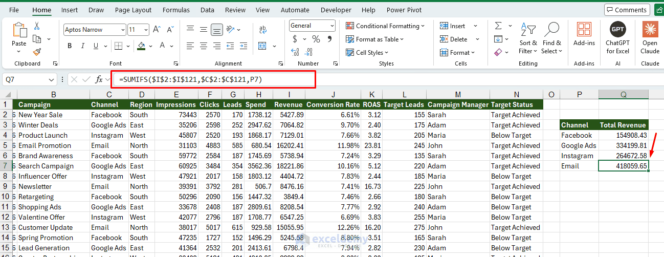
Calculate Revenue by Channel:
=SUMIFS($I$2:$I$121,$C$2:$C$121,P7)
This formula calculates the total revenue based on the channel.
Calculate Revenue Using Multiple Conditions:
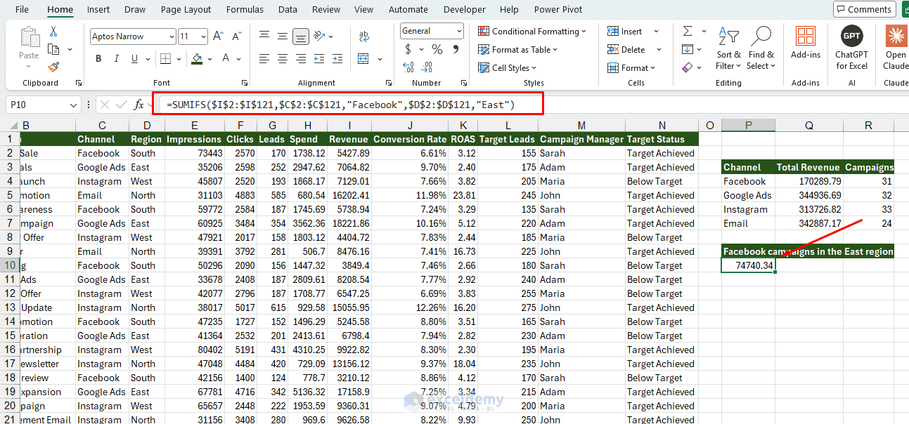
Suppose you want to calculate the revenue generated by Facebook campaigns in the East region.
=SUMIFS($I$2:$I$121,$C$2:$C$121,"Facebook",$D$2:$D$121,"East")
Excel adds revenue only when both conditions are true: the channel is Facebook and the region is East. You can also use cell references instead of typing the criteria directly.
Calculate Revenue Within a Date Range:
Place a start date in P8 and an end date in Q8, then enter:
=SUMIFS($I$2:$I$121,$A$2:$A$121,">="&P8,$A$2:$A$121,"<="&Q8)
This is useful for calculating revenue for a week, month, quarter, or custom reporting period.
3. Use COUNTIFS to Count Campaigns Meeting Multiple Conditions
The COUNTIFS function counts how many rows satisfy one or more conditions. You can use it to find how many campaigns ran on a given channel, how many leads came from particular campaigns, or how many campaigns stayed within a spending limit.
Basic Syntax:
=COUNTIFS(criteria_range1,criteria1,...)
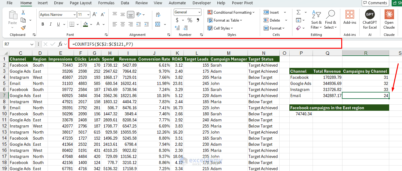
Count Campaigns by Channel:
To count how many campaigns used Facebook, enter:
=COUNTIFS($C$2:$C$121,P4)
The result is the number of rows where the Channel column contains Facebook.
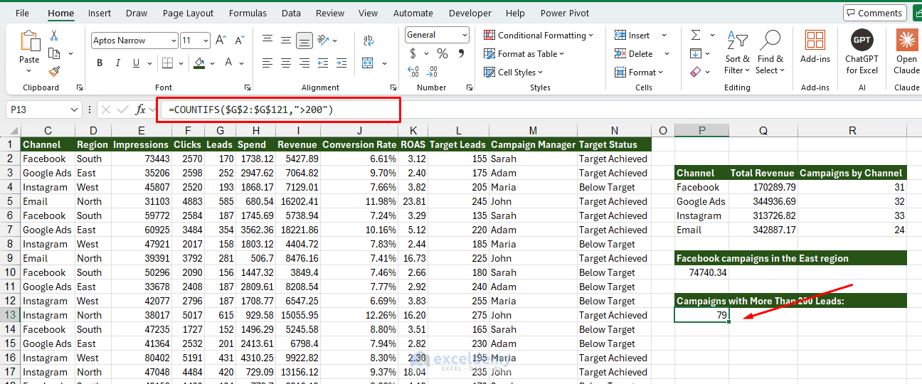
Count Campaigns with More Than 200 Leads:
=COUNTIFS($G$2:$G$121,">200")
The quotation marks are required because the criterion contains a comparison operator.
Count Campaigns Meeting Multiple Targets:
Suppose you want to count campaigns that:
- Used Google Ads
- Generated more than 200 leads
- Spent less than $2,500
=COUNTIFS($C$2:$C$121,"Google Ads",$G$2:$G$121,">200",$H$2:$H$121,"<2500")
Only campaigns satisfying all three conditions are counted.
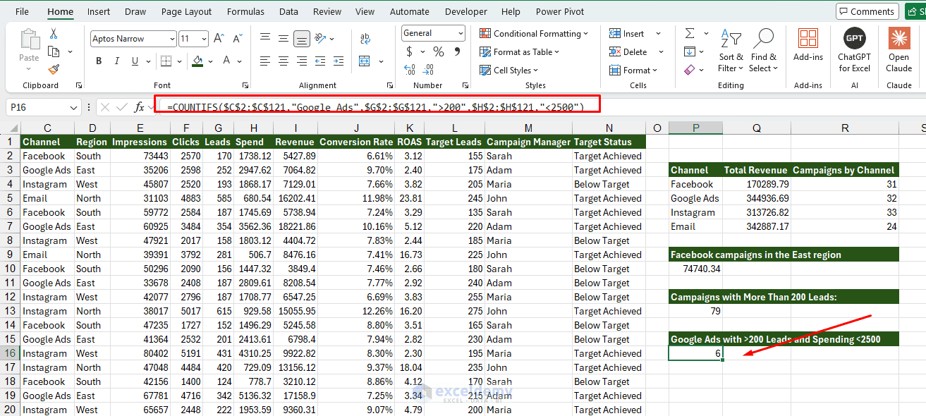
This can help marketers measure how many campaigns achieved a lead target while remaining within budget.
4. Use IF to Classify Campaign Performance
The IF function tests a condition and returns one result when the condition is true and another when it is false. You can use it to automatically label or flag data based on a rule — for example, marking a campaign as “High Performer” if it hits certain thresholds, without manually reviewing every row.
Basic Syntax:
=IF(logical_test,value_if_true,value_if_false)
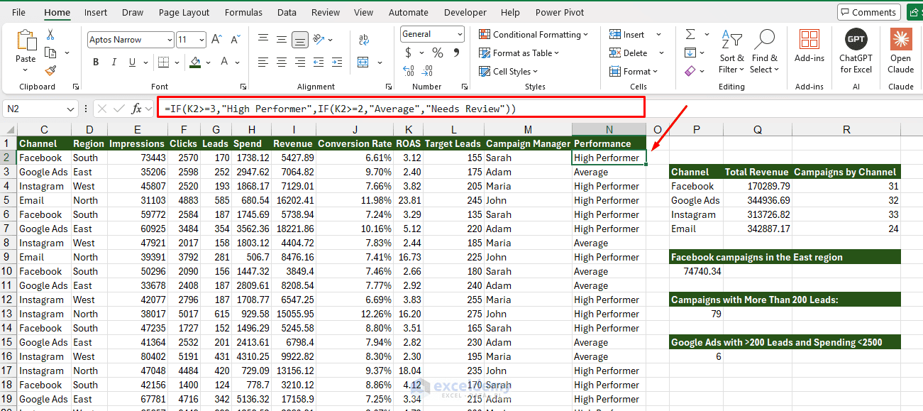
Classify Campaigns Using ROAS:
| ROAS | Classification |
| 3 or higher | High Performer |
| 2 to less than 3 | Average |
| Less than 2 | Needs Review |
=IF(K2>=3,"High Performer",IF(K2>=2,"Average","Needs Review"))
The formula checks the return on ad spend, then assigns a classification based on the score.
Check Whether a Lead Target Was Achieved:
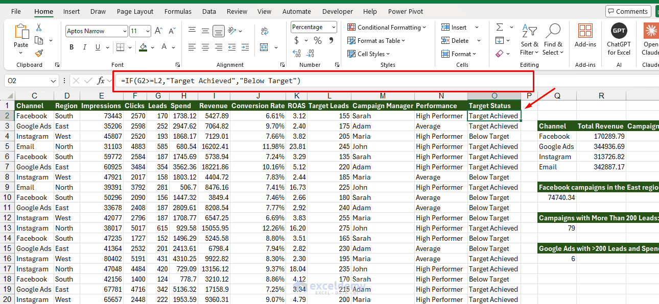
- Target Status:
=IF(G2>=L2,"Target Achieved","Below Target")
This formula compares actual leads in G2 with target leads in L2.
Flag Campaigns That Exceeded Their Budget:
Suppose the maximum permitted campaign spend is $2,000.
=IF(H2>2000,"Over Budget","Within Budget")
5. Use FILTER to Create Dynamic Campaign Reports
The FILTER function returns all rows that meet one or more conditions. Available in Microsoft 365, it creates dynamic lists that update automatically — making it ideal for dashboards. You can use it to surface high-performance campaigns, generate regional reports, review monthly performance, and more.
Basic Syntax:
=FILTER(array,include,[if_empty])
Unlike traditional filters, FILTER outputs the matching data to another part of the worksheet, and the results update automatically when the original data changes.
Filter Campaigns by Channel:
- Enter the following formula in an empty area:
=FILTER(A2:O121,C2:C121=Q4,"No campaigns found")
Excel returns every campaign where the Channel column matches the value in Q4.
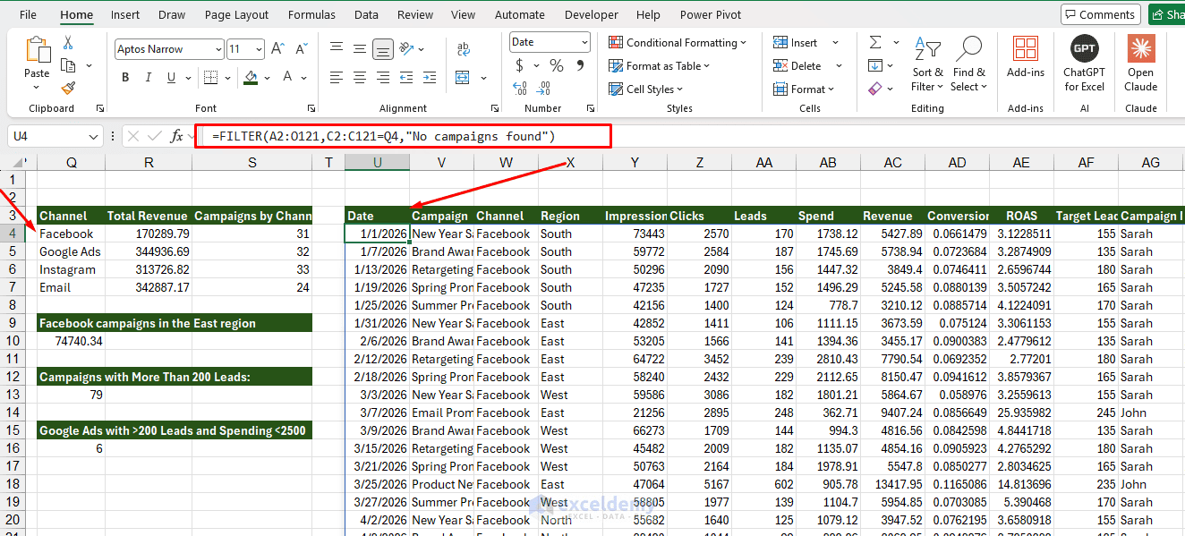
Change Q4 from Facebook to Email or Instagram, and the results will update automatically.
Filter High-Performing Campaigns:
To return campaigns with a ROAS of at least 3, enter:
=FILTER(A2:O121,K2:K121>=3,"No high-performing campaigns")
Filter Using Multiple Conditions:
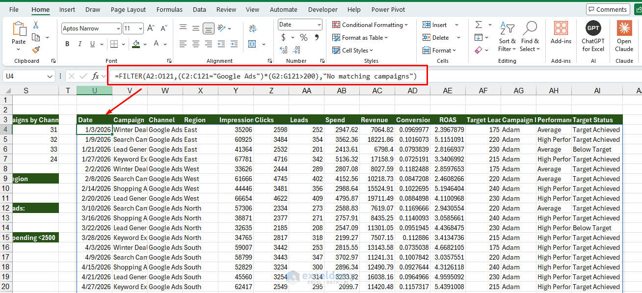
To return Google Ads campaigns with more than 200 leads, enter:
=FILTER(A2:O121,(C2:C121="Google Ads")*(G2:G121>200),"No matching campaigns")
The multiplication symbol creates AND logic, so both conditions must be true.
To return campaigns from either Facebook or Instagram, use:
=FILTER(A2:O121,(C2:C121="Facebook")+(C2:C121="Instagram"),"No matching campaigns")
The plus symbol creates OR logic, so a row is returned when either condition is true.
FILTER is a dynamic array function. Make sure the cells below and beside the formula are empty so Excel has enough space to display the results.
Bonus: TEXTSPLIT — Breaking Apart Messy Campaign Data
Marketing data is rarely clean. UTM parameters, ad names, and export files often cram multiple pieces of information into one cell — e.g. Facebook_Summer2026_Video_US. TEXTSPLIT breaks that into separate columns automatically.
Basic Syntax:
=TEXTSPLIT(text, col_delimiter, [row_delimiter], [ignore_empty], [match_mode], [pad_with])
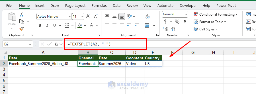
Suppose cell A2 contains: Facebook_Summer2026_Video_US
=TEXTSPLIT(A2, "_")
This spills the result across four cells: Facebook, Summer2026, Video, US — no manual splitting and no Text-to-Columns wizard required.
Real-world use case: parsing UTM campaign strings
If your utm_campaign values look like spring-sale_email_newsletter-03, you can split on multiple delimiters at once:
=TEXTSPLIT(A2, {"-","_"})
This tells Excel to split on either a hyphen or an underscore, giving you clean, individual fields for campaign, channel, and content — perfect for building a pivot table by channel afterward.
Why this beats Text-to-Columns:
Text-to-Columns is a one-time, manual operation. If your data changes, you have to redo it. TEXTSPLIT is a live formula: update the source cell, and the split values update automatically. It’s the difference between a one-off cleanup and a repeatable process.
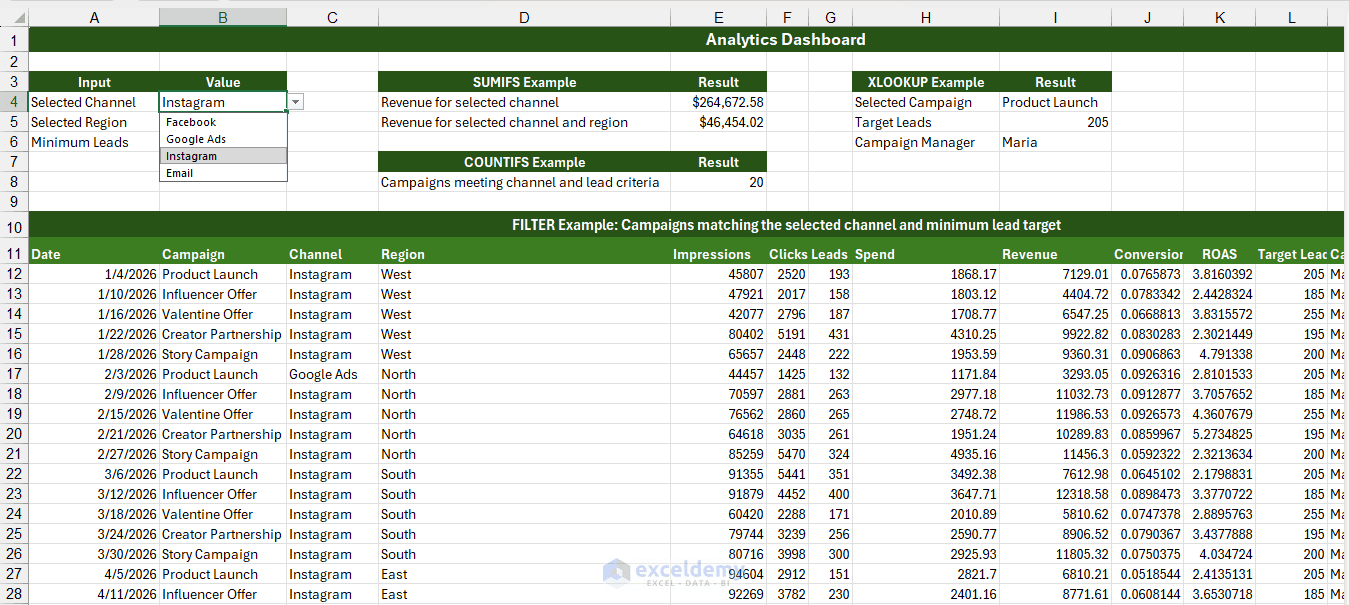
Putting It Together: A Quick Workflow Example
You can combine all of these functions to build a practical analytics dashboard.
Which Function Should You Use?
| Marketing Task | Recommended Function |
| Add revenue or spending based on conditions | SUMIFS |
| Count campaigns meeting specific requirements | COUNTIFS |
| Retrieve targets, budgets, or manager names | XLOOKUP |
| Classify or flag campaign performance | IF |
| Generate a dynamic list of matching campaigns | FILTER |
Conclusion
These five Excel functions can turn a cluttered marketing spreadsheet into a practical campaign analysis and reporting tool. Use SUMIFS to summarize revenue and spending, COUNTIFS to measure how many campaigns met your targets, and XLOOKUP to connect campaign data with targets or budgets. Use IF to classify performance and FILTER to generate dynamic reports for selected channels, regions, or performance levels.
Once these functions are combined with marketing metrics such as CTR, conversion rate, cost per lead, and ROAS, you can identify successful campaigns and find areas that need improvement — without manually reviewing every row.
Get FREE Advanced Excel Exercises with Solutions!