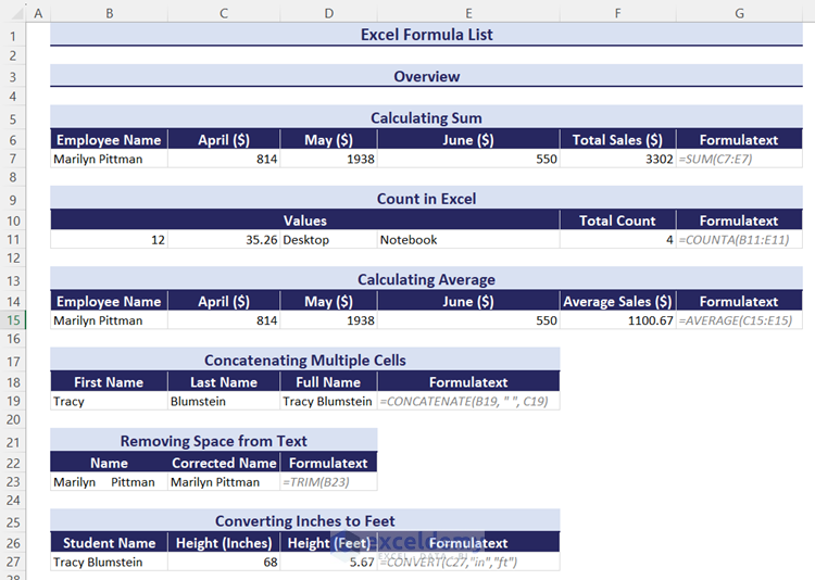
In the following image, you see some students with their marks in English. We have calculated the total marks, average marks, total no. of students, and difference between the highest and lowest marks using Excel formulas.
⏷What Is an Excel Formula?
⏷Apply Formula
⏷Add and Subtract
⏷Multiply
⏷Divide
⏷Sum
⏵AutoSum
⏵Sum Columns
⏵Sum Based on Criteria
⏷Count
⏵Count Cells
⏵Count Unique Values
⏵Count Based on Criteria
⏷Use Average Formula
⏵Average
⏵Running Average
⏵Moving Average
⏵Weighted Average
⏷Range Formula
⏷Subtotals
⏷Concatenate
⏵Multiple Cells
⏵Combine Text and Number
⏷Calculate Percentages
⏵Percentage
⏵Percentage Change
⏷Ratio
⏷Rounding
⏵Round Up Decimals
⏵Round to Nearest 5
⏷Math Formula
⏵Finding Root
⏵Multiplying Matrix
⏵Checking Even or Odd
⏷Use Text Formula
⏵Finding Text in a Cell
⏵Changing Case
⏵Removing Space
⏵Extracting Text
⏵Truncating Text
⏷Date and Time Formula
⏷Use Date and Time Functions
⏵Calculating Age
⏵Getting First Day of Month
⏵Days between Dates
⏵Calculating Time
⏷Use Conditional Formulas
⏷Use Nested Formula
⏷Use Lookup Formula
⏵Wildcard
⏵INDEX and MATCH
⏷Randomize
⏵Random Numbers
⏵Random Value from a Selection
⏷Unit Conversion
⏵Inches to Feet
⏵Kg to Lbs
⏷Serial Number Formula
⏷Some Keyboard Shortcuts for Formulas
What Is an Excel Formula?
An Excel formula is an expression that acts on a cell or range of cells and produces results in another cell or multiple cells.
How to Apply a Formula in Excel?
You can apply a formula in Excel by typing an equal sign (=) in a cell and then typing the desired formula. You can put direct values in the formula as the arguments or you can use cell references. After typing the formula, press Enter (or Ctrl + Shift + Enter for formulas that use arrays in older Excel versions) to get the desired result.
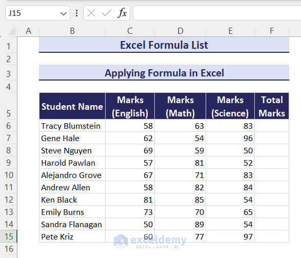
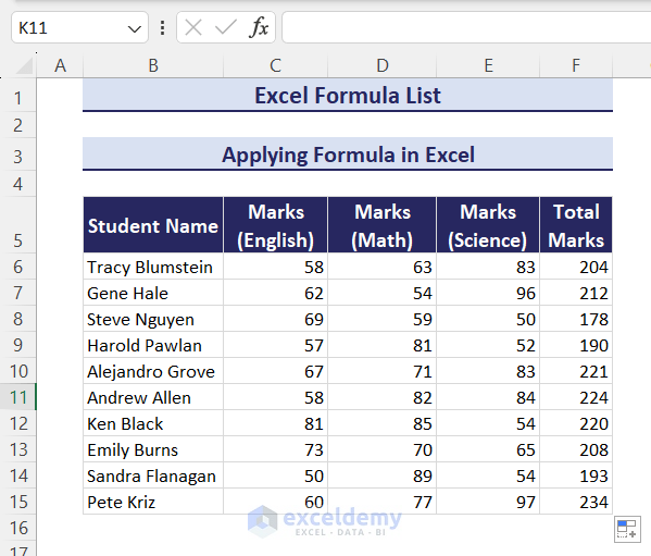
We have a dataset with some student’s marks in 3 subjects. We want to get the total marks of each student in these 3 subjects. So, we have to add the marks of these 3 subjects. We can use the SUM function here.
Follow these steps:
- Select cell F6 and type the equal sign.
- Type sum.
- Excel will suggest all the available formulas related to the sum.
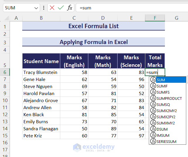
- We’ll use the SUM function here, so double-click on the SUM option.
- Click and drag over the cells from C6 to E6. You can also type the full formula.
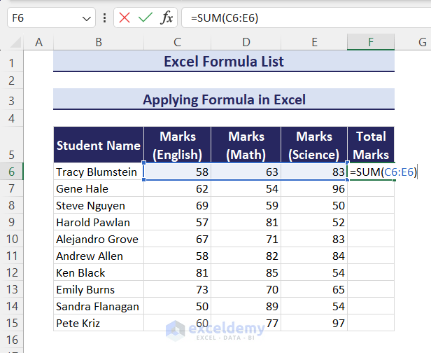
- Press Enter and you’ll get the output (total marks of the first student).
- You’ll see the Fill Handle icon located at the right bottom corner of the cell.
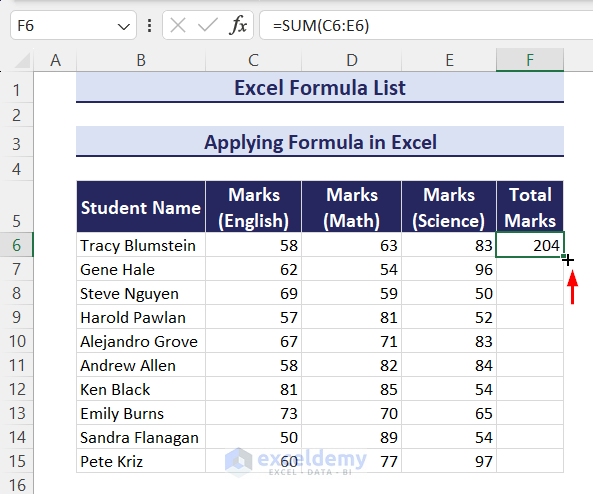
- Double-click on the Fill Handle icon or drag it down with the mouse to get the result for all students.
Part 1 – How to Add and Subtract in Excel
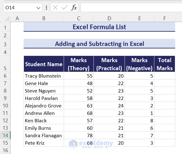
We have a dataset with some students’ marks in a subject that is divided into 3 sections (Theory, Practical and Negative). We have to add the theory and practical section’s marks and subtract the negative marks to obtain the total marks of each student.
Steps:
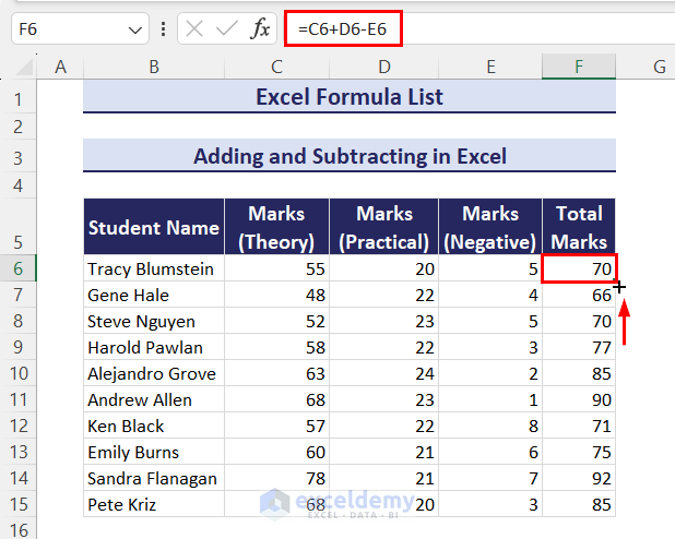
- Put the following formula in cell F6 and press Enter to get the total marks of the first student:
=C6+D6-E6- Double-click the Fill Handle icon or drag it down with a mouse to get the result for all students.
Read More: Excel GST Formula
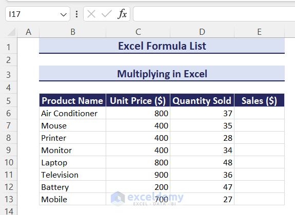
Part 2 – How to Multiply in Excel
We have a dataset with some products and their unit prices and quantity sold. We have to multiply the unit price with the quantity sold to obtain the sales of each product.
Steps:
- Apply the following formula in cell E6 to get the sales of the first product and then use the Fill Handle icon for all the remaining cells to copy the formula:
=D6*C6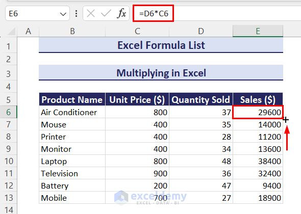
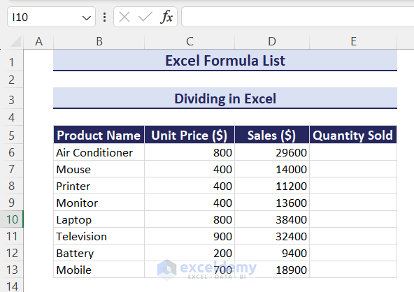
Part 3 – How to Divide in Excel
We’ll use the same dataset as before. We’ll determine the quantity sold of each product by dividing sales by unit price.
- The formula in cell E6 will be:
=D6/C6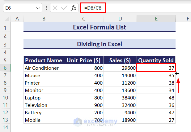
Part 4 – How to Sum in Excel
Case 4.1 – Using the AutoSum Feature
We have the following dataset with some employees and their sales in 3 different months. We want to get the sales in the employee-wise sales column.
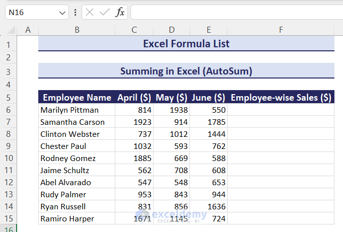
Steps:
- Select cells F6:F15.
- Go to the Home tab.
- Select the AutoSum option in the Editing group of commands.
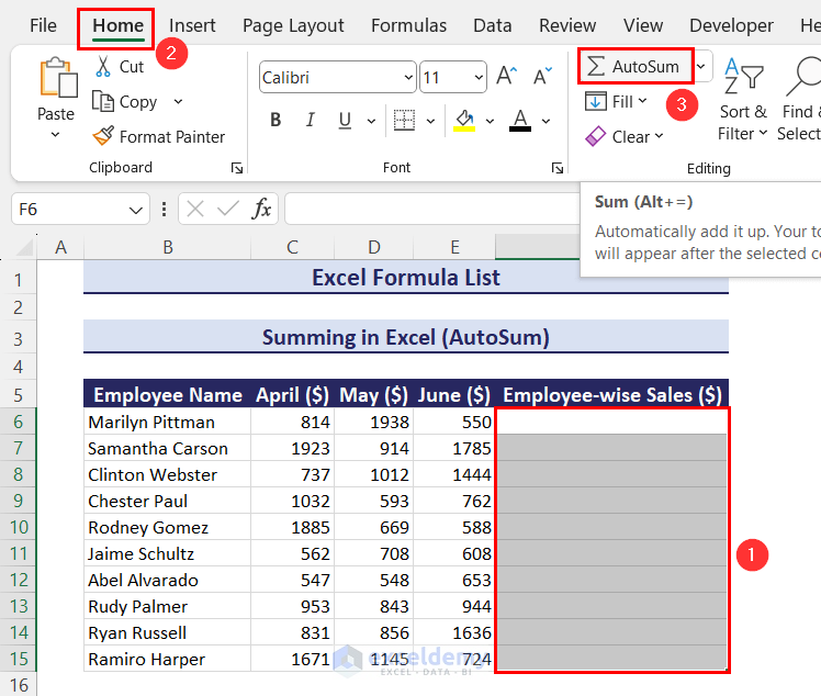
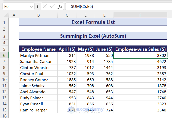
- You’ll get all the outputs together.
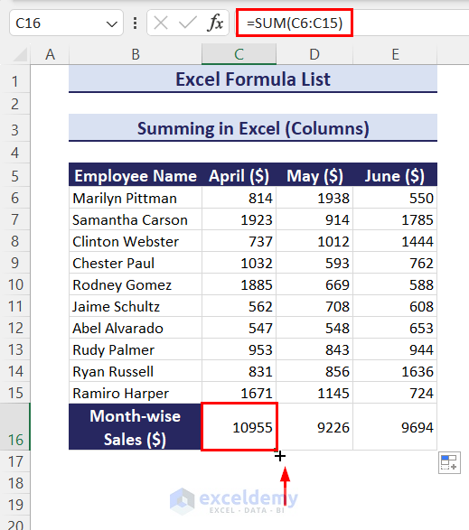
Case 4.2 – Sum Columns
We have the same employee sales dataset. We’ll calculate the total month-wise sales, so we have to sum all the columns one by one.
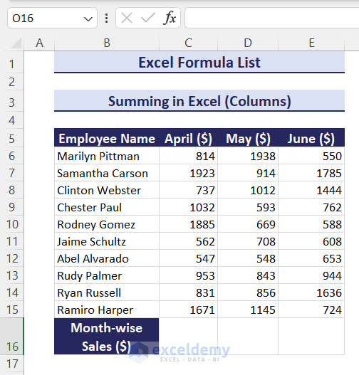
Steps:
- Use the following formula in cell C16 to get the total sales of April of all employees:
=SUM(C6:C15)- Drag the Fill Handle icon to the right for the remaining months (May and June).
Case 4.3 – Sum Based on Criteria
We have a dataset with brand names, devices, models, and their prices. We want the total price based on the two criteria below.
Criteria 1: Brand (Omicorn)
Criteria 2: Device (Notebook)
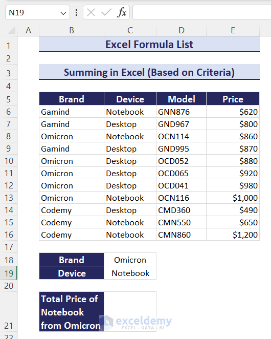
- The formula in cell C21 is:
=SUMIFS(E6:E16,B6:B16,C18,C6:C16,C19)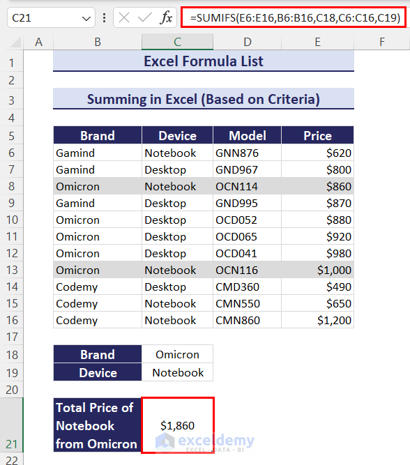
Read More: Excel Dividend Formula
Part 5 – How to Count in Excel
Case 5.1 Count Cells
We have a dataset with values like number, text, date, and empty cells.
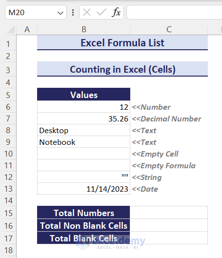
- To count numerical values, use this formula:
=COUNT(B6:B13)- To count numerical values, texts, and formulas, use this:
=COUNTA(B6:B13)- To count blank cells, use this formula:
=COUNTBLANK(B6:B13)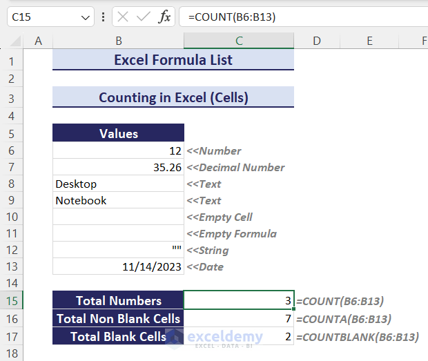
Case 5.2 – Count Unique Values
We have a dataset with brand names, devices, models, and their prices. We want to count the unique brands and unique devices separately.
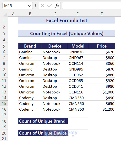
- Use this formula in cell D18 to count the unique brands:
=COUNTA(UNIQUE(B6:B16))- Put this formula in cell D20 to count the unique devices:
=COUNTA(UNIQUE(C6:C16))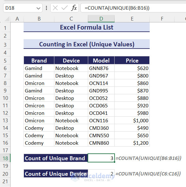
Case 5.3 – Count Based on Criteria
We have the same dataset. We want the total count based on the criteria below.
Criteria 1: Brand (Omicorn)
Criteria 2: Device (Notebook)
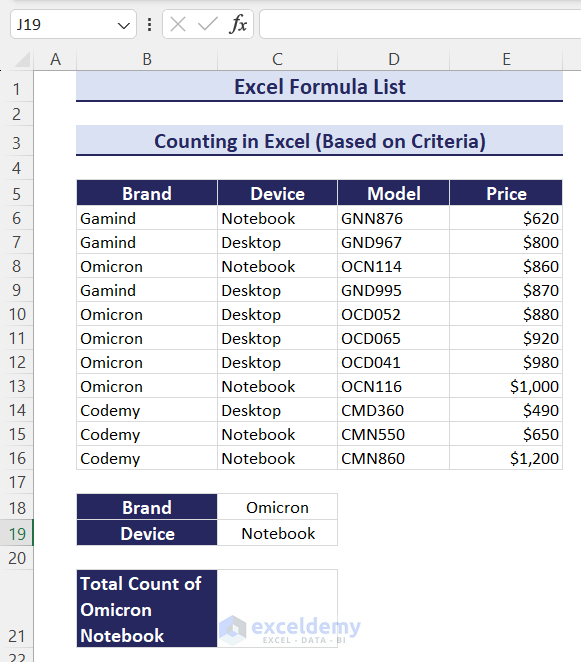
- The formula is:
=COUNTIFS(B6:B16,C18,C6:C16,C19)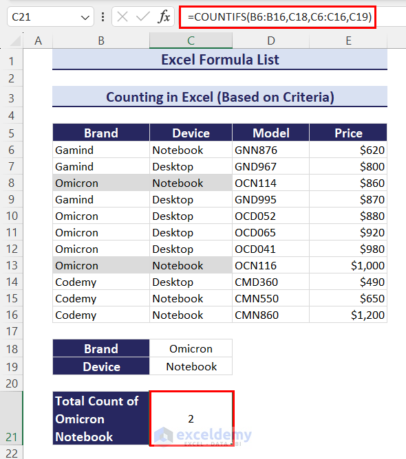
Read More: How to Calculate Discount in Excel
Part 6 – How to Use the Average Formula in Excel
The basic formula for calculating the average is:
Average = Sum of All Values / Number of ValuesCase 6.1 – Calculate the Average
We have the following dataset with some employees and their sales in 3 different months. We want to get the average sales of each employee in average sales column.
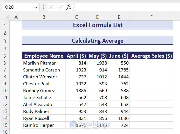
Steps:
- Insert the following formula in cell F6 to get the average sales of the first employee and then use the Fill Handle icon for all the remaining cells to copy the formula:
=AVERAGE(C6:E6)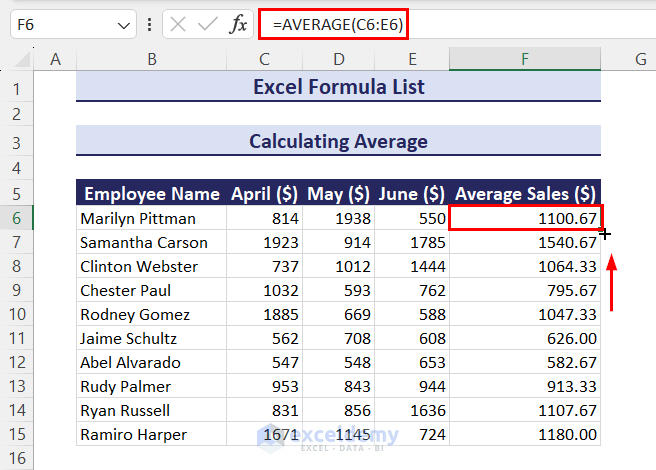
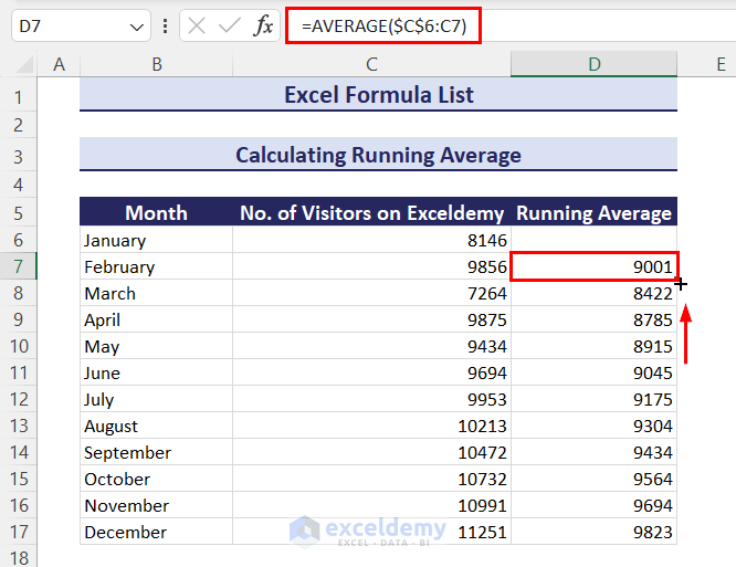
Case 6.2 – Running Average
A running average is a type of average that is continually updated as new data points become available. We have the following dataset with months and no. of visitors on the Exceldemy forum. We want to calculate the running average of the no. of visitors in each month starting from the second month.
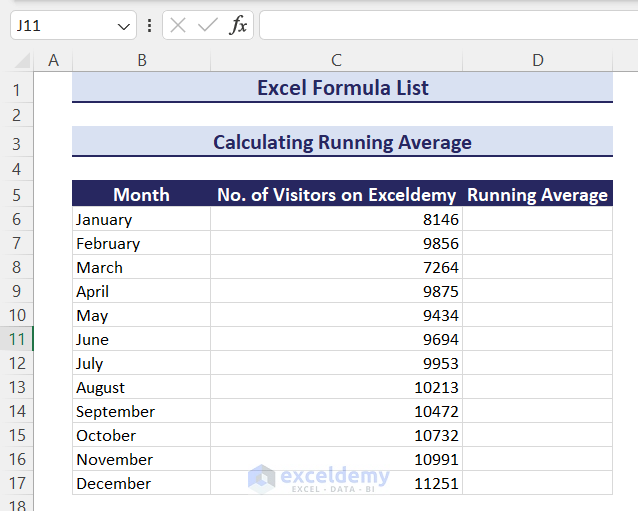
Steps:
- Use the following formula in cell D7 and press Enter to get the running average of the first two months:
=AVERAGE($C$6:C7)- Double-click the Fill Handle icon or drag it down with a mouse to get the result for all months.
Case 6.3 – Moving Average
A moving average is a type of average that continually updates the average as new data points are added or old data points are removed.
We have the same dataset as before. We want to calculate the 3-points moving average of the no. of visitors.
Steps:
- Use the following formula in cell D8 to get the 3-point moving average of the no. of visitors and then use the Fill Handle icon for all the remaining cells:
=AVERAGE(C6:C8)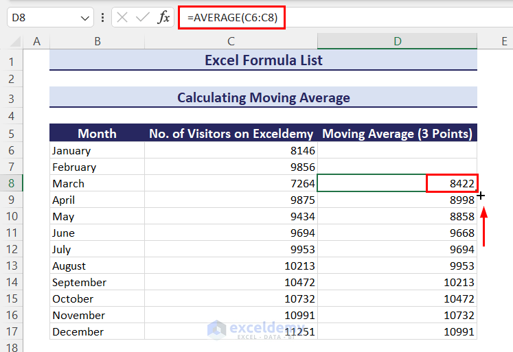
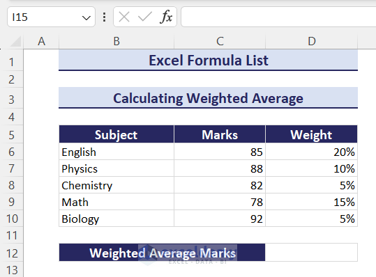
Case 6.4 – Weighted Average
The weighted average is an average in which each data point is assigned a weight based on its relative importance in the overall set.
We have the following dataset of a student’s marks in some subjects and the weights assigned to each subject. We want to calculate the weighted average marks.
- The formula to calculate the weighted average marks is:
=SUMPRODUCT(C6:C10,D6:D10)/SUM(D6:D10)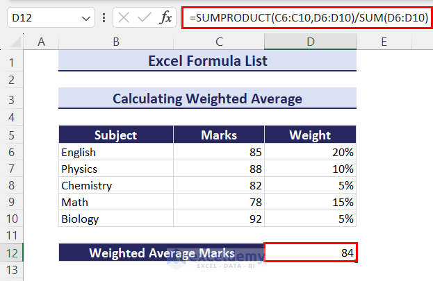
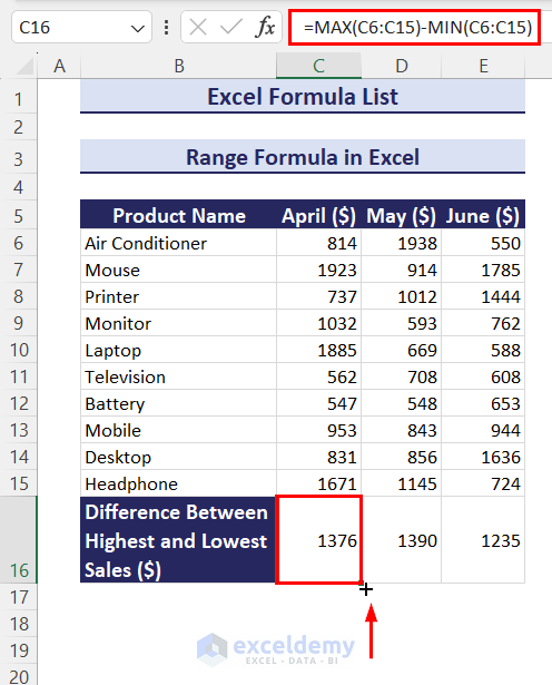
Part 7 – Range Formulas in Excel
We have the following dataset where we have some products and their sales in 3 different months. We want to get the difference between the highest and lowest sales in each month.

Steps:
- Put the following formula in cell C16 to get the difference between the highest and lowest sales in April:
=MAX(C6:C15)-MIN(C6:C15)- Drag the Fill Handle icon to the right for May and June.
Part 8 – Subtotals in Excel
We have a dataset with some products, unit price, quantity sold and their sales values. There are 3 common products. We want to calculate the subtotal sales of those 3 products one by one and then their grand total sales.
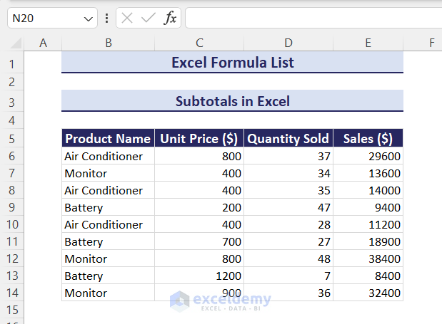
We have to make the dataset like below by sorting the same products together.
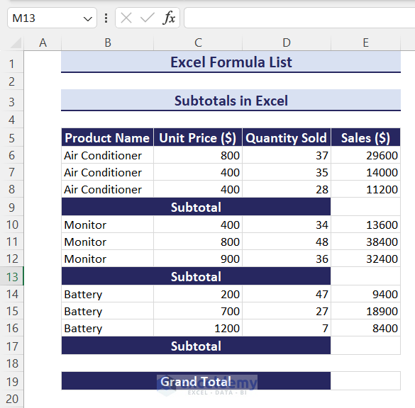
Steps:
- Insert the following formula in cell E9 to get the subtotal sales of the Air Conditioner:
=SUBTOTAL(9,E6:E8)The first argument of the SUBTOTAL function is function_num. This argument denotes the function we want to use in our calculation. We have used 9 because 9 denotes the SUM function.
- Repeat for Monitor in cell E13:
=SUBTOTAL(9,E10:E12)- Use the formula for Battery in cell E17:
=SUBTOTAL(9,E14:E16)- Insert the following formula in cell E19 to get the grand total sales of all products:
=SUBTOTAL(9,E6:E17)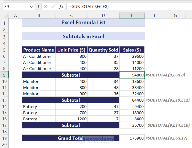
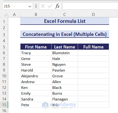
Part 9 – Concatenate in Excel
Example 1 – Concatenate Multiple Cells
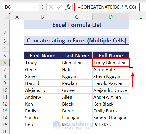
Here’s a dataset with some people’s first names and last names in 2 separate cells in 2 columns. We want to concatenate the values from these 2 cells to obtain the full name.
Steps:
- Use the following formula in cell D6 and press Enter to get the full name by joining the first and the last name with a space:
=CONCATENATE(B6, " ", C6)- Double-click the Fill Handle icon or drag it down with a mouse to get the result for all people.
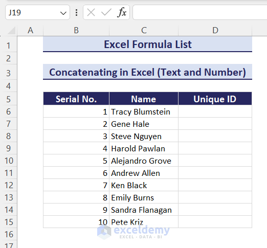
Example 2 – Combine Text and Number
We have another dataset with some employees’ names and their serial numbers. We want to join this text and number to form unique IDs for all the employees.
Steps:
- Put the following formula in cell D6 to combine the serial number and name and then use the Fill Handle icon for all the remaining cells:
=B6&"-"&C6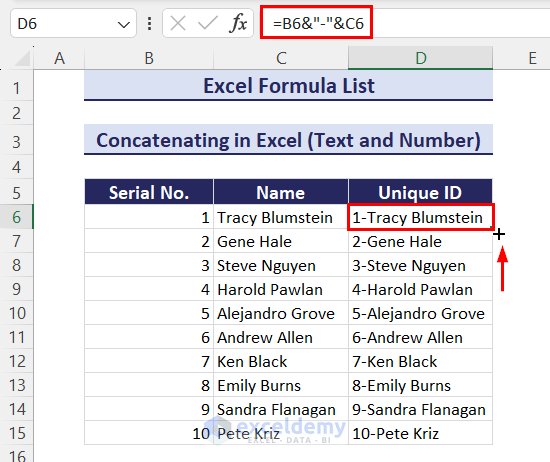
Part 10 – How to Calculate Percentages in Excel
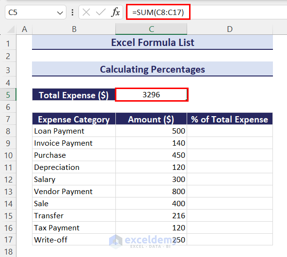
The percentage of a part can be calculated by dividing it by the total value and then multiplying the result by 100 or formatting the result with the Percent Style command.
Example 1 – Calculate Percentages
We have a dataset with individual expense categories and their amounts. We have calculated the total expense using the SUM function and want to find the individual category expense in % of the total expense.
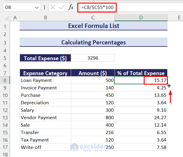
Steps:
- Insert the following formula in cell D8 to get the Loan Payment expense in % of the total expense:
=C8/$C$5*100- Drag the Fill Handle icon down to obtain percentages for all the category expenses.
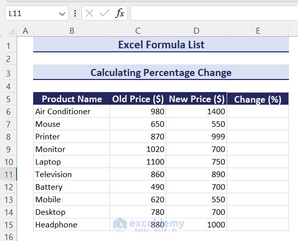
Example 2 – Calculate the Percentage Change
We have a dataset of some products and their old and new prices. We want to calculate the percentage change of the old prices.
- Use the following formula to get the percentage change:
=(D6-C6)/C6*100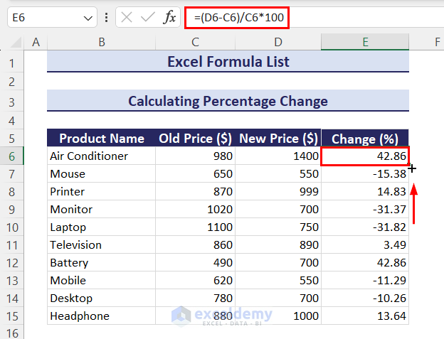
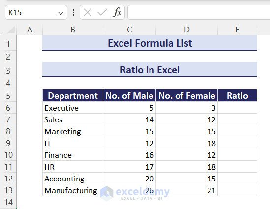
Part 11 – Ratios in Excel
Consider a dataset with some departments of a company. We have a number of male and female workers in those departments. We want to get the male-female ratio in each department.
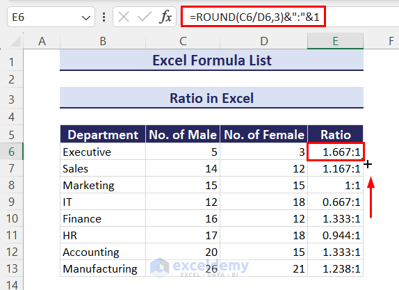
Steps:
- Use the following formula in cell E6 to get the male-female ratio in the Executive department:
=ROUND(C6/D6,3)&":"&1- Drag the Fill Handle icon down to obtain the male-female ratios for all the departments.
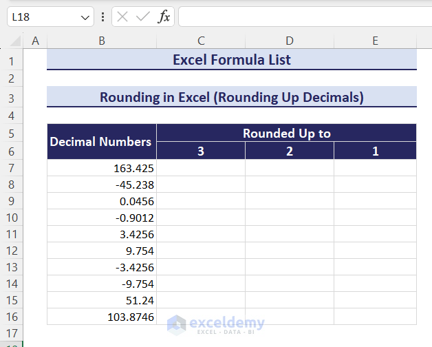
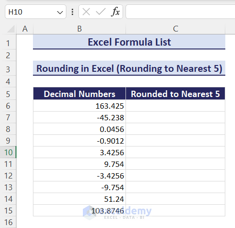
Part 12 – Rounding in Excel
Case 12.1 – Round Up Decimals
We have some decimal numbers (both positive and negative). We want to round them up to 3, 2, and 1 decimal places.
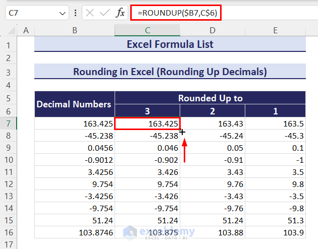
Steps:
- Use the following formula in cell C7 and press Enter to get the first number rounded up to 3 decimal places:
=ROUNDUP($B7,C$6)- Double-click the Fill Handle icon or drag it down to round up all numbers to 3 decimal places.
- With the range in column C selected, drag the fill handle from C17 to the right round up all numbers to 2 and 1 decimal places, respectively.
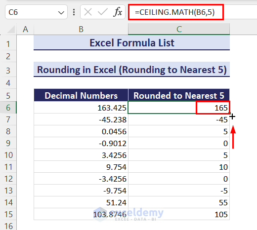
Case 12.2 – Round to Nearest 5
We have the same dataset as before. We’ll use the CEILING.MATH function to round these numbers to the nearest 5. Note: The CEILING.MATH function is available from Excel 2013 or later versions.
Steps:
- Use the following formula in cell C6 to round the first number to the nearest 5:
=CEILING.MATH(B6,5)- Drag the Fill Handle icon down to round all numbers to the nearest 5.
Part 13 – Math Formulas in Excel
Case 13.1 – How to Find the Root
We have a list of numbers (both positive and negative). We’ll calculate the square root of these numbers using the SQRT function.
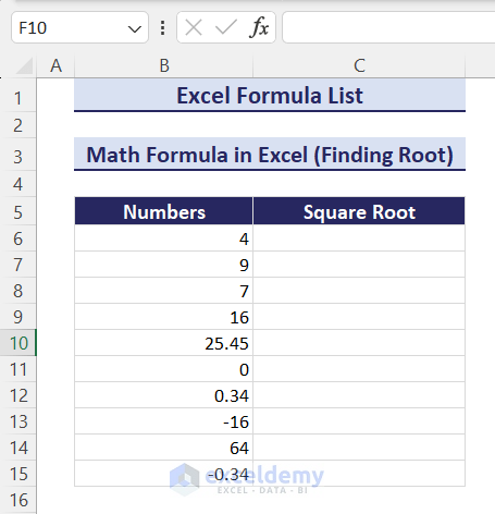
- The formula to put in cell C6 is:
=SQRT(B6)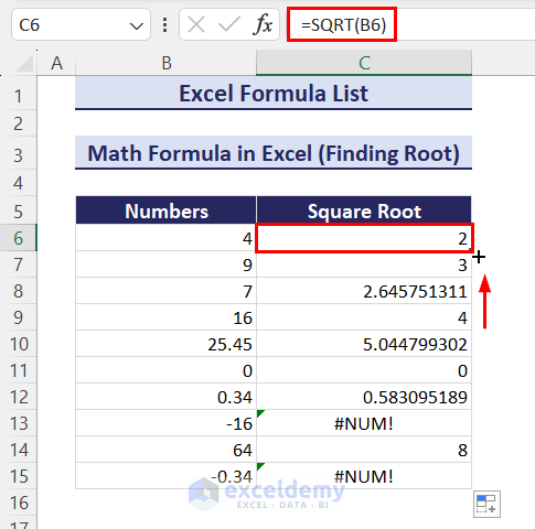
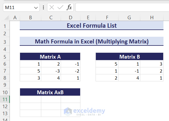
Case 13.2 – How to Multiply a Matrix
When multiplying matrices (arrays), both arrays must only contain numbers, and the number of rows in array2 and the number of columns in array1 must be the same.
We have a dataset with 2 matrices, Matrix A and B. Both have 3 rows and 3 columns.
Steps:
- Insert the following formula in cell B11 and press Enter to get the product of 2 matrices:
=MMULT(B6:D8,F6:H8)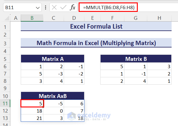
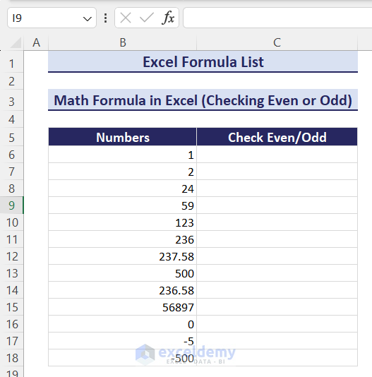
Case 13.3 – Check for Even or Odd
We have a list of numbers. To check even or odd, we’ll use the combination of IF and ISEVEN functions.
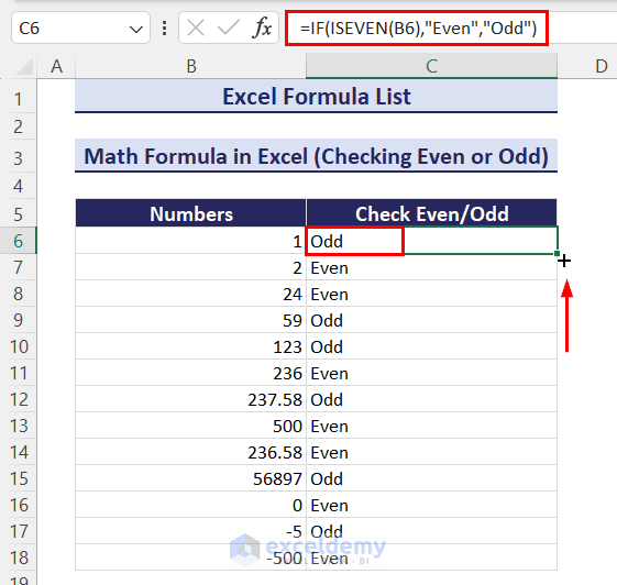
Steps:
- Use the following formula in cell C6 to check if the number is even:
=IF(ISEVEN(B6),"Even","Odd")- Drag the Fill Handle icon down to check all the numbers.
Read More: Excel Sales Formula
Part 14 – How to Use Excel Text Formulas
Case 14.1 – Find Text in a Cell
We have a list of email IDs and want to find Gmail among those email IDs. You can use the SEARCH function to find the starting position of Gmail from the left side of an email ID. The ISNUMBER function will check whether the position is a number or not.

- The formula is:
=IF(ISNUMBER(SEARCH($C$5,B6)),"Yes","No")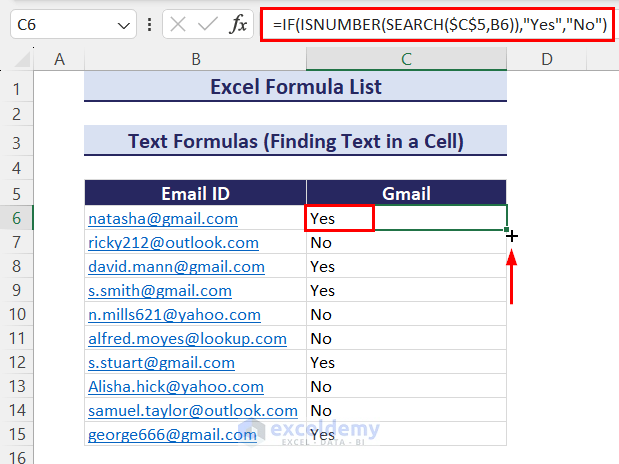
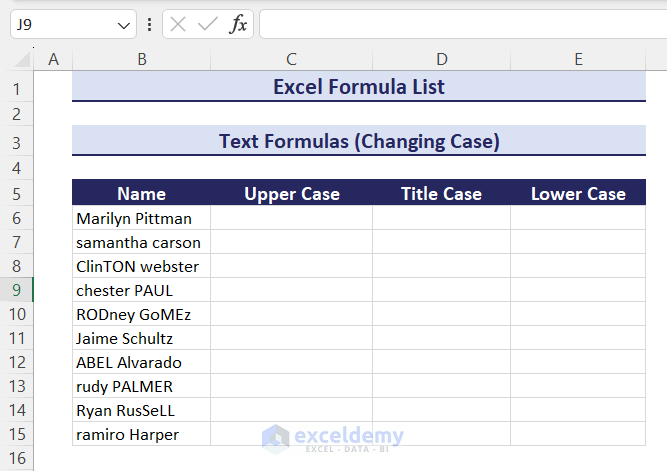
Case 14.2 – Change the Text Case
We have a list of names that aren’t in the correct cases.
- Use the following formula in cell C6 to change the case to upper case:
=UPPER(B6)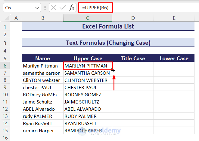
- Use the following formula in cell D6 to change the case to the title case:
=PROPER(B6)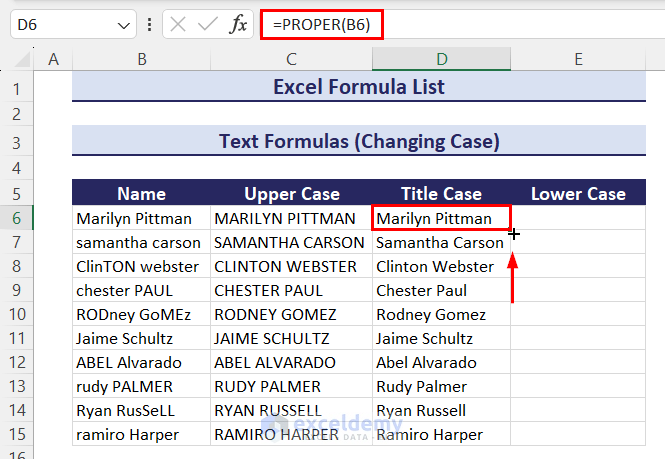
- Insert the following to get the lower case in cell E6:
=LOWER(B6)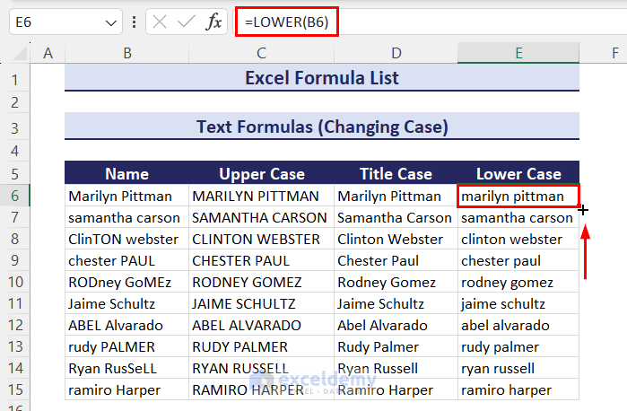
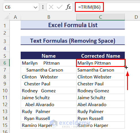
Case 14.3 – Remove Space
We have a dataset of some names having 2 parts (first and last name), but there are unnecessary spaces between first and last names, as well as before and after the name.
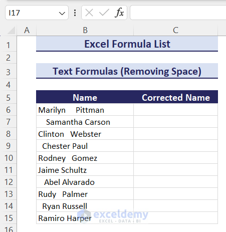
Steps:
- Put the following formula in cell C6 to remove extra spaces from the name:
=TRIM(B6)- Drag the Fill Handle icon down to remove spaces from all names.
Case 14.4 – Extract Text
We have a dataset with some products and their codes. The product codes are in 3 parts separated by hyphens. We want to extract the first, middle, and last parts of these codes.
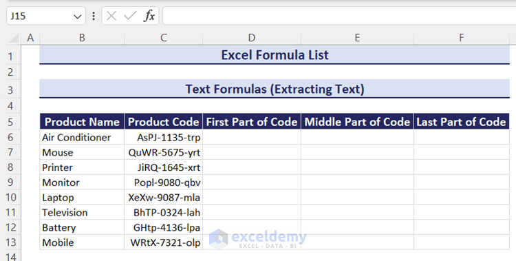
- To extract four characters from the left side (first part of the code), use this formula:
=LEFT(C6,4)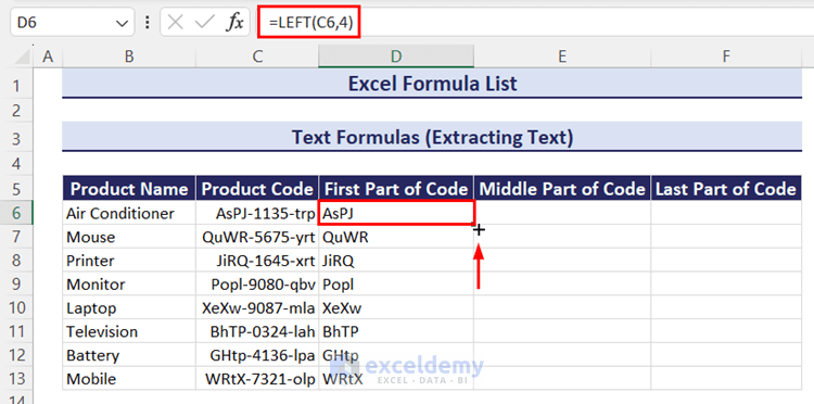
- To extract four characters from the middle, starting at position 6 (middle part of the code), use this formula:
=MID(C6,6,4)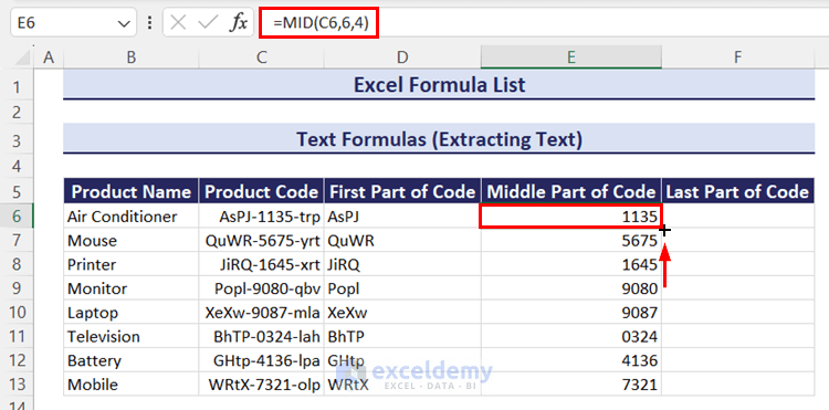
- For extracting three characters from the right side (last part of the code), use the following:
=RIGHT(C6,3)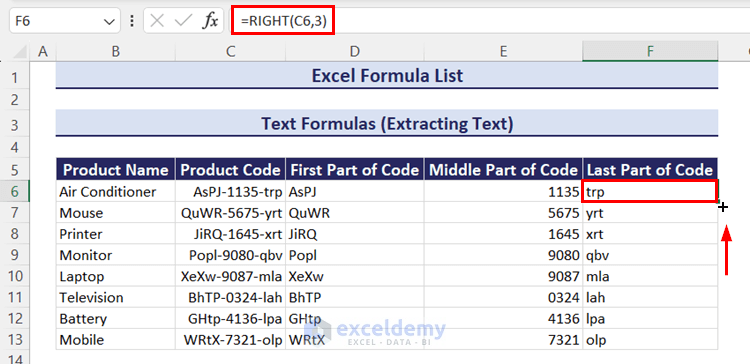
Case 14.5 – Truncate Text
We have a list of unique IDs of some employees of a company. The IDs are made with serial numbers and employee’s names. We want to truncate the IDs and replace them with the names of the employees.
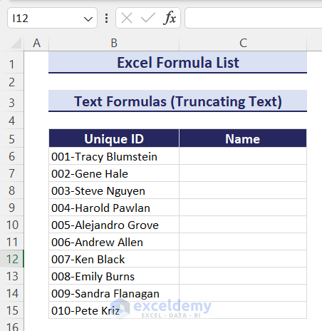
- The formula given below will replace the unique IDs with the employee’s names:
=REPLACE(B6,1,4,"")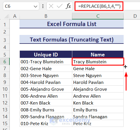
Part 15 – Date and Time Formula in Excel
We’ll see how various functions calculate date and time with the following simple dataset.

- To get today’s date only, use any of these formulas:
=TODAY()=DATE(YEAR(TODAY()),MONTH(TODAY()),DAY(TODAY()))- You can also put the date of your choice using this formula:
=DATE(2023,11,16)- To get today’s date and time together, use this formula:
=NOW()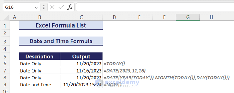
Read More: Excel Scoring Formula
Part 16 – How to Use Date and Time Functions in Excel
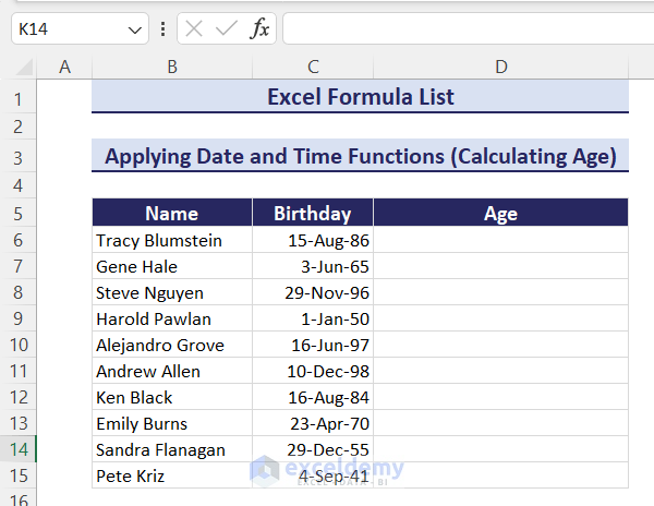
Case 16.1 – Calculate Age
We have a list of birthdays of some people and want to calculate their age as of today.
We’ll take the birthday as the starting date and use the TODAY function to get today’s date as the ending date.
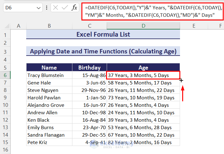
Steps:
- Insert the following formula in cell D6 and press Enter to get the age of the first person:
=DATEDIF(C6,TODAY(),"Y")&" Years, "&DATEDIF(C6,TODAY(),"YM")&" Months, "&DATEDIF(C6,TODAY(),"MD")&" Days"- Double-click the Fill Handle icon or drag it down to get the result for all people.
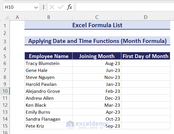
Case 16.2 – Get the First Day of the Month
We have a list of some employees and their joining month which is in Date format. We want to know the first day of their joining month.
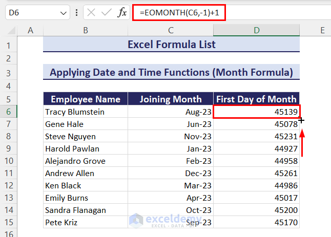
We’ll use the EOMONTH function to get the serial number for the last day of the previous month before the joining date.
Steps:
- Use the following formula in cell D6 and press Enter to get the serial number for the first day of the joining month:
=EOMONTH(C6,-1)+1- Double-click the Fill Handle icon or drag it down to get the result for all employees.
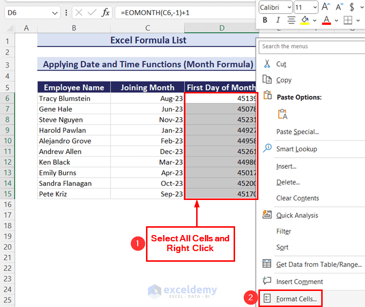
- Select all cells D6:D15.
- Right-click to open the Context menu.
- Choose Format Cells.
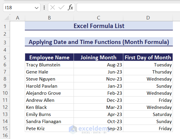
- The Format Cells window will open.
- Go to the Number tab.
- Choose Custom under Category.
- Type or choose dddd in the box.
Tips: The keyboard shortcut for opening the Format Cells window is Ctrl + 1.

- Click the OK button to apply the format. You’ll get the first day of the joining month.
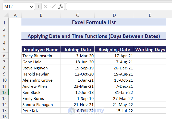
Case 16.3 – Days Between Dates
We have some employees’ joining date and resigning date in a project. We want to know the number of working days of each employee.
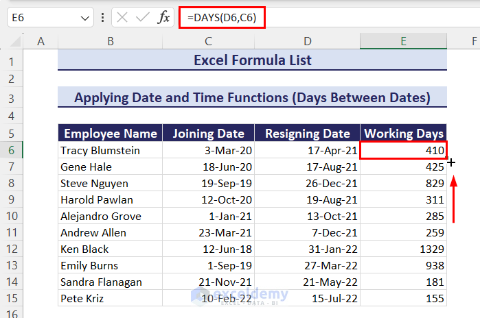
Steps:
- Use the following formula in cell E6 to calculate the working days of the first employee:
=DAYS(D6,C6)- Drag the Fill Handle icon down to calculate the working days of all employees.
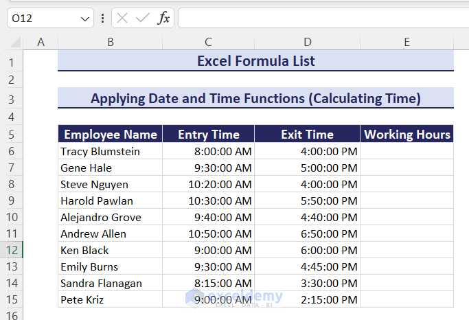
Case 16.4 – Calculate Time
We have a similar kind of dataset but now we have entry time and exit time of employees. We want to calculate the working hours.
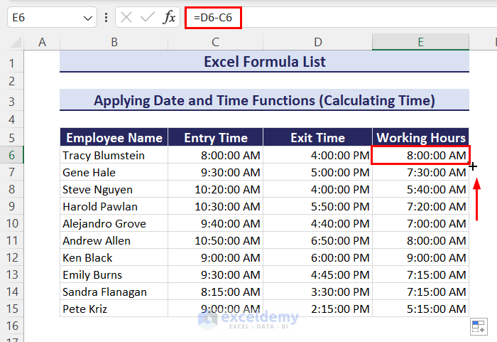
Steps:
- Put the following formula in cell E6 and press Enter to calculate the working hours of the first employee:
=D6-C6- Double-click the Fill Handle icon or drag it down with a mouse to calculate the working hours of all employees.
You’ll see AM after working hours because the cell is in Time format. When we subtract one time from another time, the resulting cell automatically becomes a Time-formatted cell.
- Select cells E6:E15.
- Right-click to open the Context menu.
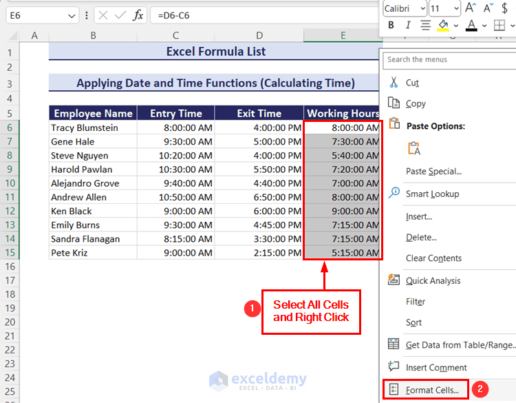
- Click on the Format Cells option, and the Format Cells window will open.
- Go to the Number tab.
- Choose Custom under Category.
- Type or choose h:mm:ss.
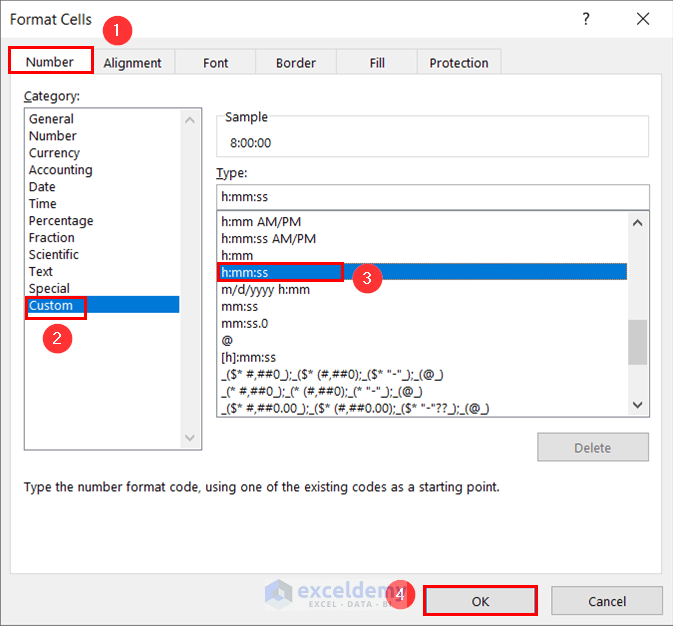
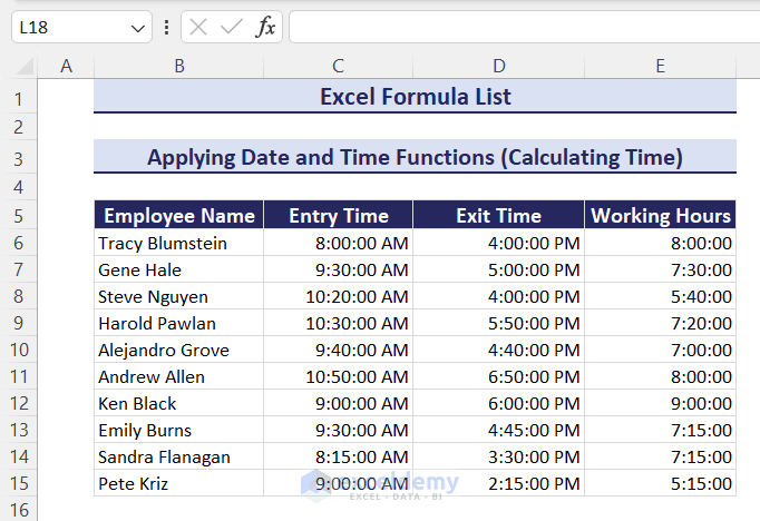
- Click the OK button to apply the format. You’ll get the working hours for all the employees.
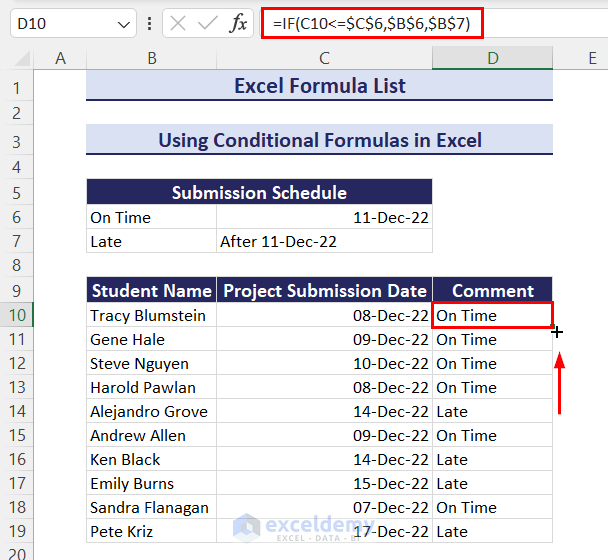
Part 17 – How to Use Conditional Formulas in Excel
We have a dataset with some students and their project submission date and want to make a comment based on the submission date. If the submission date is on or before 11 Dec, the comment is On Time. If the submission date is after 11 Dec, the comment becomes Late. These values have been put in the table for references.
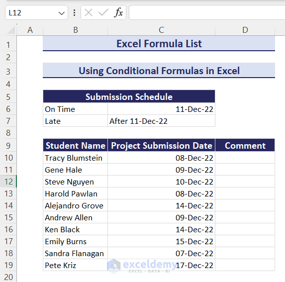
Steps:
- Insert the following formula in cell D10 to make a comment for the first student:
=IF(C10<=$C$6,$B$6,$B$7)- Drag the Fill Handle icon down to make comments for all.
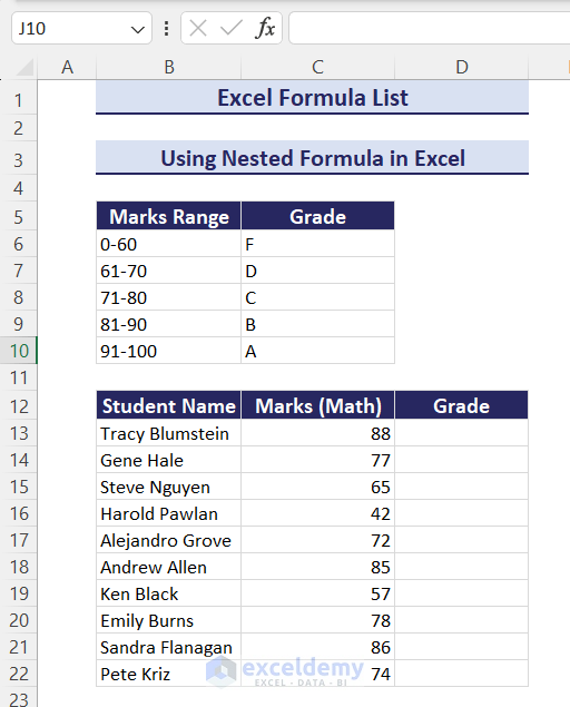
Part 18 – How to Use a Nested Formula in Excel
A nested formula is when you use one function as an argument inside another function. We already showed simple examples of nesting above.
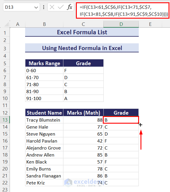
We have a student marksheet in Math and the marks range for 5 grades. We want to assign a grade to each student.
Steps:
- Use the following formula in cell D13 and press Enter to assign a grade to the first student:
=IF(C13<61,$C$6,IF(C13<71,$C$7,IF(C13<81,$C$8,IF(C13<91,$C$9,$C$10))))- Double-click the Fill Handle icon or drag it down to assign all grades.
Read More: Excel Overtime Formula
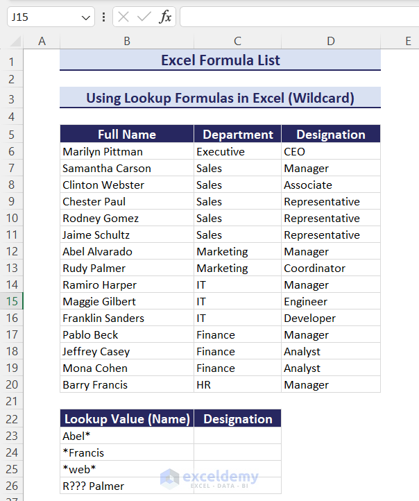
Part 19 – How to Use Lookup Formulas in Excel
Case 19.1 – Wildcards for Partial Matches
The asterisk wildcard (*) replaces any number of characters (including 0) after a text, before a text, and both before and after a text. The question mark wildcard (?) finds only the number of characters based on the number of question marks. If there is a single question mark wildcard, it’ll search for a single character.
We have an employee database with names, departments, and designations. You can see 4 lookup values (names) here. We put the asterisk wildcard after a name, before a name, and both before and after a name. We have also put the question mark wildcard 3 times between a name. We’ll partially search for these values in the database and extract the matching designation using the VLOOKUP function.
- Use the following formulas for partial matching based on wildcard:
=VLOOKUP(B23,B6:D20,3,FALSE)=VLOOKUP(B24,B6:D20,3,FALSE)=VLOOKUP(B25,B6:D20,3,FALSE)=VLOOKUP(B26,B6:D20,3,FALSE)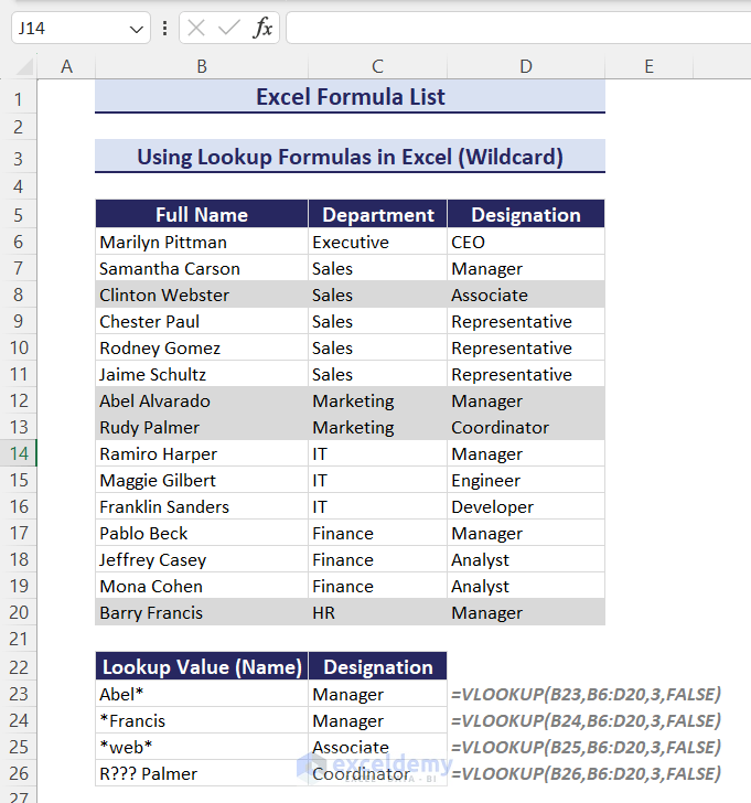
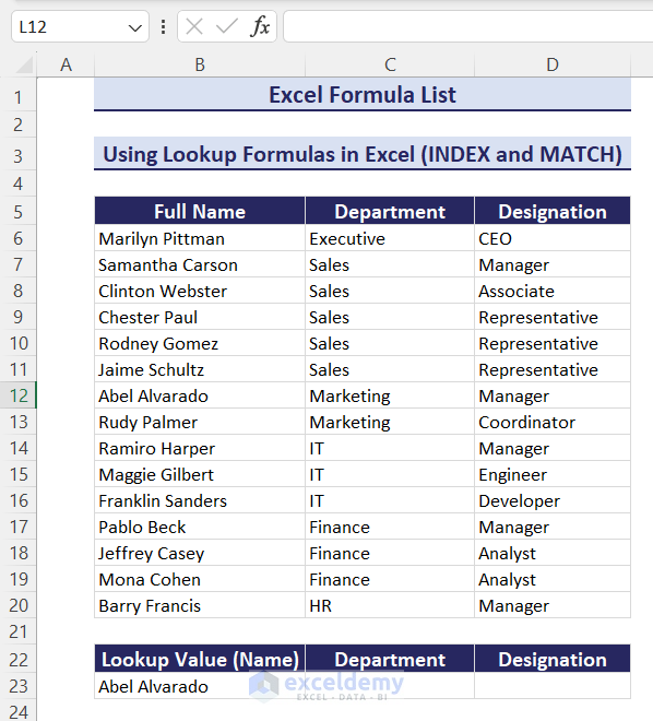
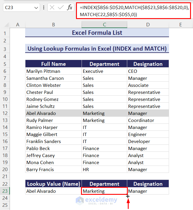
Case 19.2 – INDEX and MATCH for Exact Matches
We have the same employee database. We’ll search for a name in the database and extract the department and designation of that person.
Steps:
- Use the following formula in cell C23 to get the department based on the name:
=INDEX($B$6:$D$20,MATCH($B$23,$B$6:$B$20,0),MATCH(C22,$B$5:$D$5,0))- Drag the Fill Handle icon to the right side for designation.
Part 20 – Randomize in Excel
Case 20.1 – Generate Random Numbers
We have a dataset with lower and upper limits. We’ll generate random numbers between them.
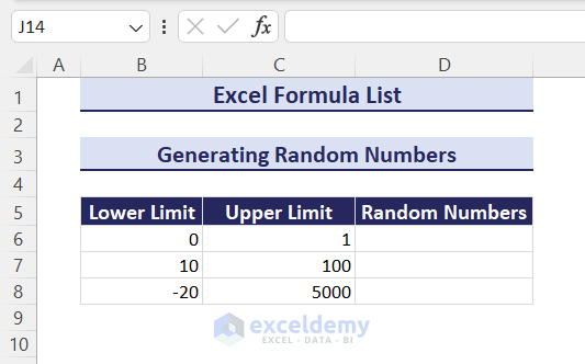
- To generate random numbers between 0 to 1, use this formula:
=RAND()- To generate random numbers between lower and upper limits, use these formulas:
=RANDBETWEEN(B7,C7)=RANDBETWEEN(B8,C8)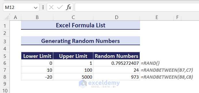
- Use the following formula to generate an array of random integers based on no. of rows, no. of columns, lower limit, and upper limit:
=RANDARRAY(B6,C6,D6,E6,TRUE)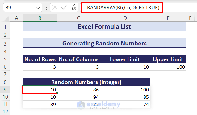
- Use the following formula to generate an array of random decimals based on no.of rows, no. of columns, lower limit, and upper limit:
=RANDARRAY(B6,C6,D6,E6,FALSE)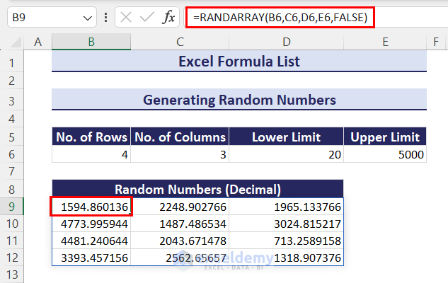
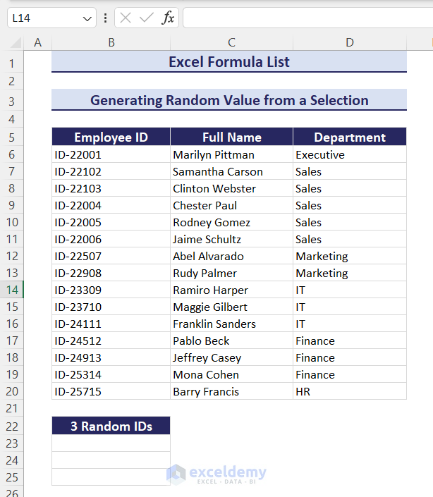
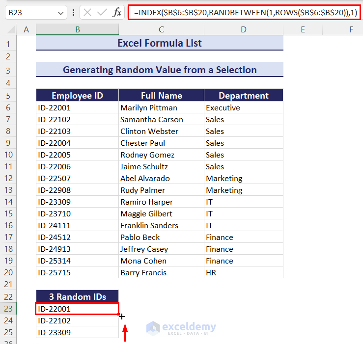
Case 20.2 – Generate a Random Value from a Selection
We have an employee database with IDs, names, and departments. We want to generate a random selection of 3 IDs from all. The purpose can be a lottery.
Steps:
- Put the following formula in cell B23 to generate a random ID:
=INDEX($B$6:$B$20,RANDBETWEEN(1,ROWS($B$6:$B$20)),1)The ROWS function will give all the row numbers of IDs. The RANDBETWEEN function generates a random row number from all row numbers. The INDEX function will extract that random ID based on the row number.
- Drag the Fill Handle icon down to generate more random IDs.
Read More: Ageing Formula in Excel
Part 21 – Unit Conversion in Excel
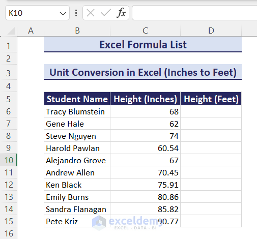
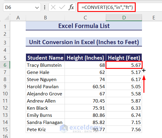
Example 1 – Convert Inches to Feet
We have some student’s heights in inches.
Steps:
- Insert the following formula in cell D6 to convert the height of the first student from inches to feet:
=CONVERT(C6,"in","ft")- Drag the Fill Handle icon down to convert all remaining values.
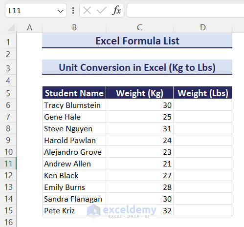
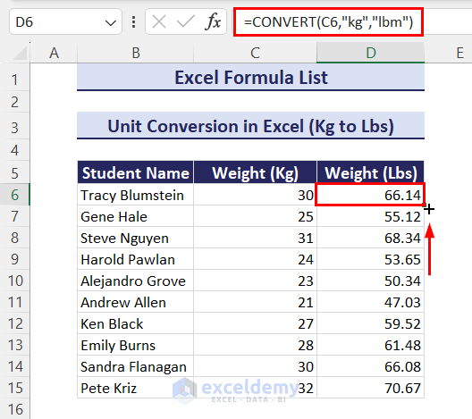
Example 2 – Convert kg to lbs
We have some student’s weights in kg.
Steps:
- Use the following formula in cell D6 to convert the weight of the first student from kilograms to pounds:
=CONVERT(C6,"kg","lbm")- Use the Fill Handle icon to convert all remaining values.
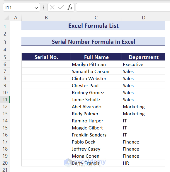
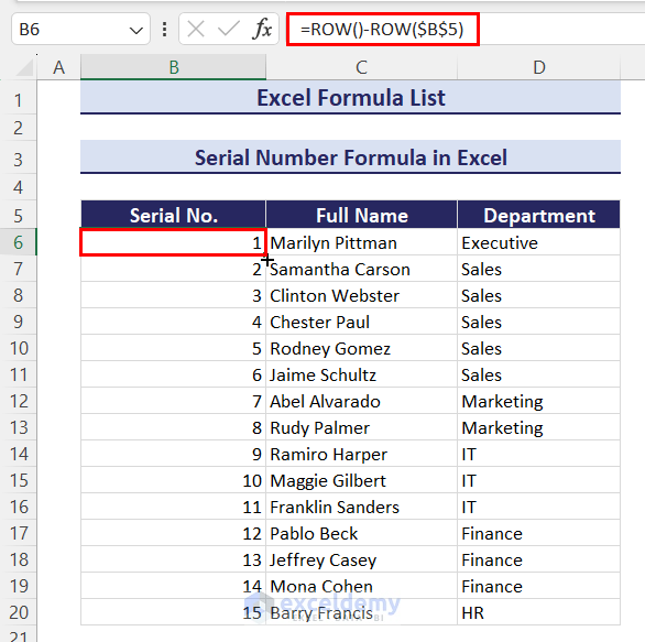
Part 22 – Serial Number Formula in Excel
We have a dataset with some employees’ names and departments. We want to put serial numbers in column B.
Steps:
- Use the following formula in cell B6 and press Enter to get the first serial number:
=ROW()-ROW($B$5)- Double-click the Fill Handle icon or drag it down to get all serial numbers.
Some Keyboard Shortcuts and Features
| Keyboard Shortcuts/Features | Tasks |
|---|---|
| F4 | Toggle between absolute, relative, and mixed references |
| Ctrl + ~ | Show all formulas on the sheet |
| F2 | Edit a formula |
| Select a formula and press F9 | Debug formulas |
| Fill Handle tool | Copy a formula to all cells in a column or row |
| Ctrl + C | Copy cells with the formula |
| Ctrl + V | Paste cells with the formula |
| Shift + F10 + V | Paste Special (Values Only) |
Download the Practice Workbook
Excel Formula List: Knowledge Hub
<< Go Back to Learn Excel
Get FREE Advanced Excel Exercises with Solutions!
