How to Create a Scoring Formula in Excel (System, Text, Grade, Z Score)

Scoring formulas in Excel are valuable for ranking and evaluating datasets. They allow us to calculate scores efficiently, consider weights, rewards, and penalties. Let’s explore how to create scoring systems using various functions.

Scoring System Requirements

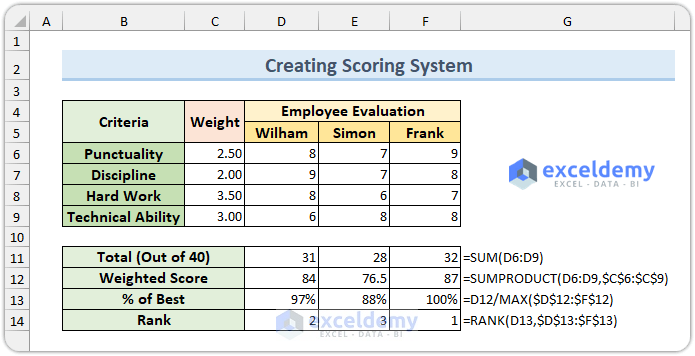
To build an Excel scoring system, you’ll need four key formulas:

• Total Score (SUM Function):

• Weighted Average Score (SUMPRODUCT Function):

• Percentile Calculation (MAX Function):

• Employee Ranking (RANK Function):

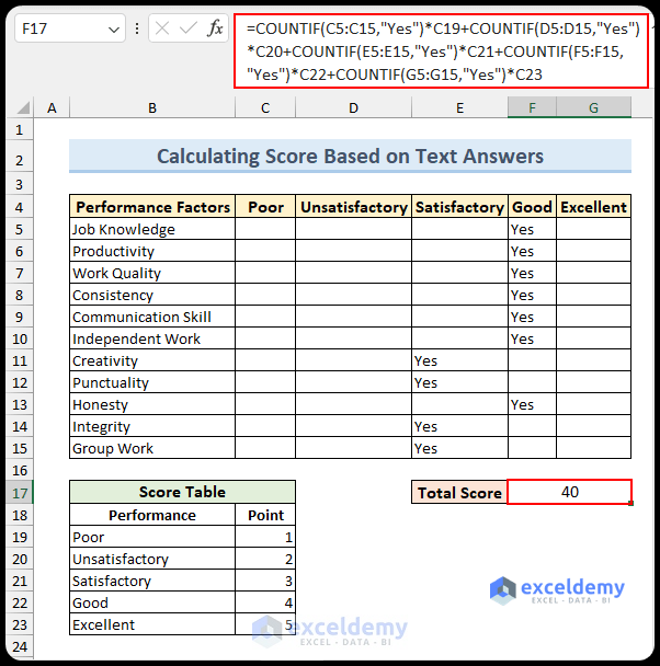
Text-Based Scoring Formula

For text-based answers, use the COUNTIF function to create the following formula (applied in cell F17):

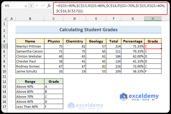
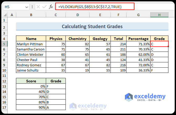
Grade Calculation in Excel

1. Using the IF Function

• To determine students’ grades, apply the IF function:

Read More: How to Create a Scoring System in Excel

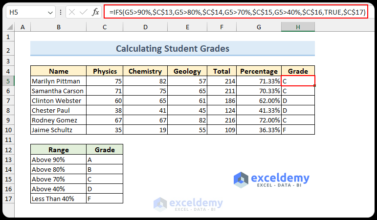
2. Using the IFS Function

• Alternatively, insert the IFS function for grade calculation:

3. VLOOKUP for Grade Scores

• Use the VLOOKUP function to find grade scores:

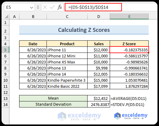
Z Score Calculation

When comparing values to the average and variability of a group, the Z score enhances accuracy.  Follow these steps:

• Calculate the average (cell D13):

• Compute the standard deviation (cell D14):

• Find the Z score using this formula:

Read More: How to Calculate T Score in Excel

Things to Remember

• If using numbers instead of percentages, adjust the criteria accordingly.
• For greater than or less than comparisons, include equal signs (i.e., <= or >=).
• Named ranges can simplify VLOOKUP formulas.
• Be cautious when working with nested IF formulas; close all parentheses properly.

Download Practice Workbook

You can download the practice workbook from here:

Frequently Asked Questions

1. How to rank values based on multiple criteria in Excel?

To rank based on multiple criteria in Excel, you can utilize the RANK function in conjunction with either the SUMPRODUCT or COUNTIF function. Here’s an example:

The RANK function calculates the rank number from the range $C$5:$C$15 based on the value in cell C5. This accounts for duplicate values in cells C10 and C11 (resulting in a rank number of 2). The SUMPRODUCT function handles situations where there are tied values, returning 0 when there are none and 1 when there is a tie. Notably, the double negative operator (—) is used to convert TRUE/FALSE results into 1/0, respectively. This formula effectively avoids duplicate rank numbers.

2. How to apply conditional formatting in the scoring formula in Excel?

Conditional formatting can be applied through the Home tab. Select your data and navigate to the Conditional Formatting option in the Styles group. From there, you’ll find various options to apply conditional formatting. For instance, you can highlight the top ten percent values by selecting Top 10% from the Top/Bottom Rules.

3. How to incorporate bonus or penalty in the scoring formula in Excel?

To incorporate bonuses or penalties into a scoring formula, first, outline the criteria for adding or deducting points. Then, use the IF function to integrate these criteria into the main scoring system. You may need to create an additional column to accommodate this adjusted scoring system.

Excel Scoring Formula: Knowledge Hub

<< Go Back to Formula List | Learn Excel