What is a Scoring Matrix and Where Do We Use It?
A scoring matrix is a valuable tool for assessing the relative worth of various items, such as jobs, projects, or properties. It allows governance teams to evaluate factors like cost, risk, and potential financial returns. Additionally, scoring matrices are useful for assessing student performance or employee demonstrations.
Step 1 – Define Criteria for the Scoring Matrix
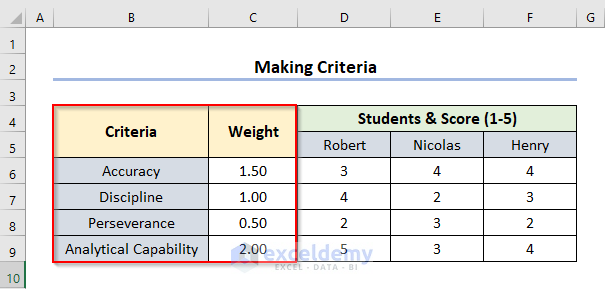
- Create a column header labeled Criteria.
- Define four criteria: Accuracy, Discipline, Perseverance, and Analytical Capability.
- Assign weights to each criterion (e.g., 1.50, 1.00, 0.50, and 2.00, respectively) within a total weight of 10.
- Enter student scores (e.g., Robert, Nicolas, and Henry) for each criterion (scores range from 1 to 5).
The dataset showing Criteria and Score:
Step 2 – Calculate Total Scores
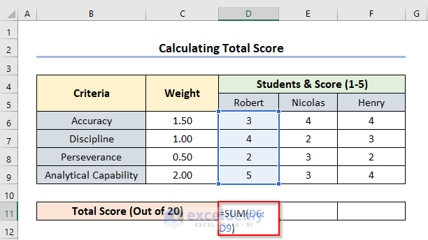
- Calculate the total score for each student.
- For Robert, enter the formula in cell D11:
=SUM(D6:D9)-
- This sums up Robert’s scores for Accuracy, Discipline, Perseverance, and Analytical Capability.
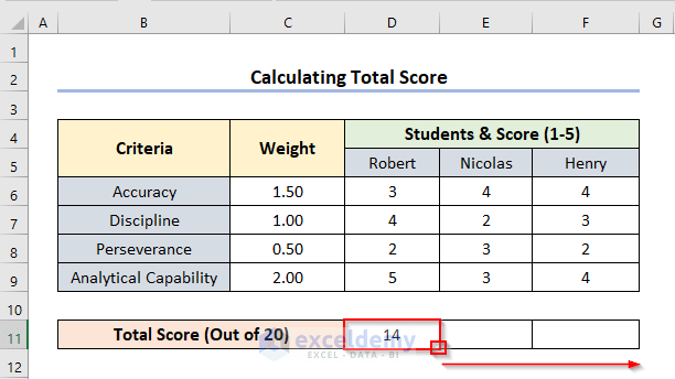
- Press ENTER to find the output as 14.
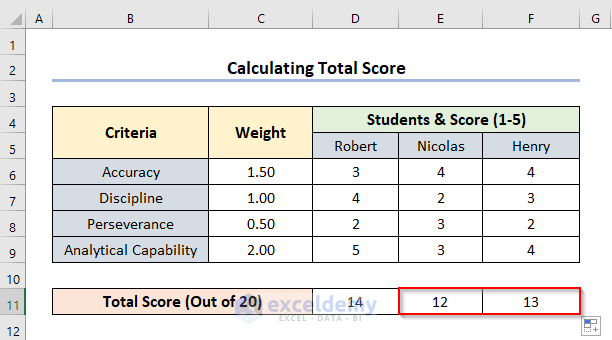
- Drag the fill handle to compute scores for the other students.
Step 3 – Compute Weighted Scores
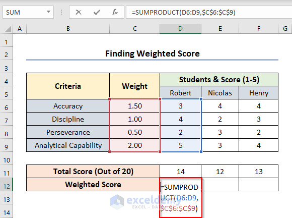
- Use the SUMPRODUCT function to find the weighted score for each student.
- For Robert, enter the formula in cell D12:
=SUMPRODUCT(D6:D9,$C$6:$C$9)-
- This calculates the weighted sum of scores based on the assigned weights.
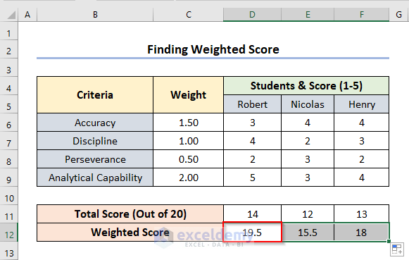
Formula Explanation:
- SUMPRODUCT(D6:D9,$C$6:$C$9) → returns the sum of D6*C6, D7*C7, D8*C8, D9*C9, i.e. (1.50*3 + 1.00*4 + 0.50*2 + 2.00*5)
- Output → 19.5
- Press ENTER and drag the Fill Handle to compute the weighted scores for all students.
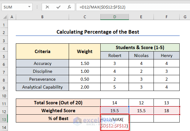
Step 4 – Determine Percentage of the Best
- Calculate the percentage of the best score for each student.
- For Robert, enter the formula in cell D13:
=D12/MAX($D$12:$F$12)-
- This divides Robert’s weighted score by the maximum weighted score.
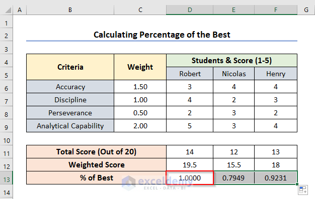
Formula Explanation:
- MAX($D$12:$F$12) → returns the maximum value among cells D12, E12, F12 E. among 19.5, 15.5, 18.
- Output → 5
- D12/MAX($D$12:$F$12) → returns the output of division between 5 and 19.5.
- Output → 1.0000
- Press ENTER and drag the Fill Handle to compute percentages for the other students.
Step 5 – Assign Ranks
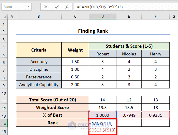
- Determine the rank for each student using the RANK function.
- For Robert, enter the formula in cell D14:
=RANK(D13,$D$13:$F$13)-
- This ranks Robert’s percentage among the other students.
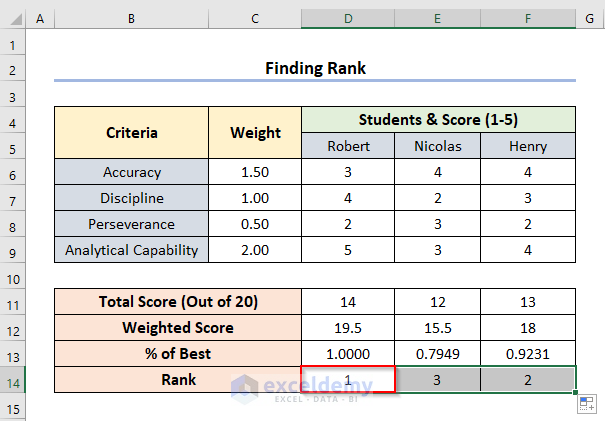
- Press ENTER and drag the Fill Handle to assign ranks to all students.
Download Practice Workbook
You can download the practice workbook from here:
<< Go Back to Scoring | Formula List | Learn Excel
Get FREE Advanced Excel Exercises with Solutions!
