How to Create a Leaderboard in Excel (with Easy Steps)

The procedures to create a leaderboard in Excel in this tutorial can also be used to create any type of dataset to rank a list of data.

Step 1 – Making a Base Excel Dataset

Lets create the base dataset which we will then update to create a leaderboard in Excel.

STEPS:

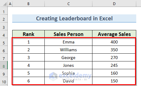
Create a simple data table as in the image below and type in the names of the sales persons.

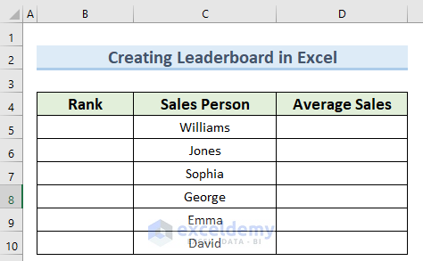
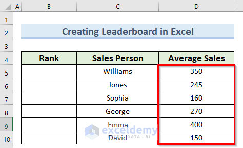
Enter some values for the Average Sales for each sales person.

Step 2 – Inserting ROW Function

Now let’s generate the rank values to create the salesperson leaderboard using the ROW function.

STEPS:

Go to cell B5 and enter the following formula:

=ROW()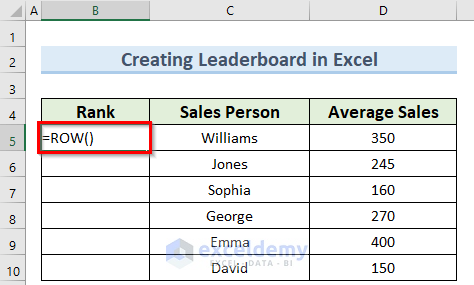

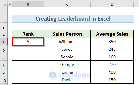
Press Enter to confirm the formula, which will return the row number in cell B5.

Step 3 – Modifying the ROW Formula

We now a value of 5 as the starting rank, which is not what we want, because we want to start our ranking with 1. Let’s modify the formula to accomplish this.

STEPS:

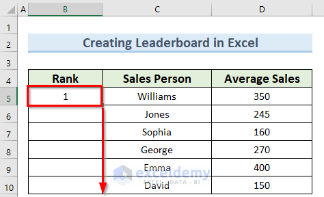
Navigate to cell B5 and enter the formula below:

=ROW()-4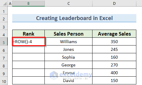

Press Enter.
Copy the formula to the other cells using the Fill Handle.

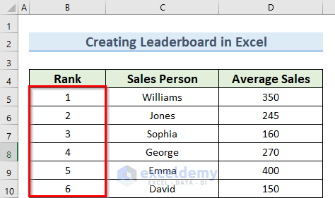
You should now have the ranking numbers in ascending order.

Step 4 – Sorting Performance Values

Now let’s sort the average sales values to create the leaderboard.

STEPS:

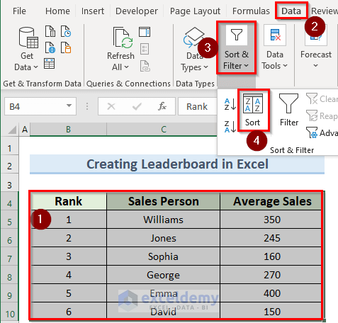
Select the whole data table.
Go to the Data tab.
Click on Sort under Sort & Filter.

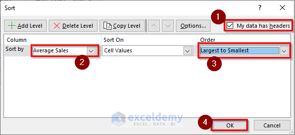
In the Sort window that opens:

Check the My data has headers box.
Select Average Sales from the Sort by drop-down option.
Select Largest to Smallest under the Order drop-down option.
Click OK.

The sales persons should now be ranked according to their Average Sales values.

Things to Remember

The ROW function yields the row number of the cell containing the formula when no reference is given.
We can specify a cell or a range of cells as the argument of the ROW function.
In Excel 365, which supports dynamic array formulae, the outcome is an array of size {4,5,6} that spills vertically into three cells, starting with the cell that contains the formula.
To get column numbers, you can similarly use the COLUMN function.
To count the number of rows, use the ROWS function.

Download Practice Workbook

Create a Leaderboard.xlsx

<< Go Back to Scoring | Formula List | Learn Excel

Get FREE Advanced Excel Exercises with Solutions!

Private Sub Worksheet_Change(ByVal Target As Range) Dim AffectedRange As Range If Not Intersect(Target, Me.Columns("D")) Is Nothing Then Set AffectedRange = Me.Range("D5:D" & Me.Cells(Me.Rows.Count, "D").End(xlUp).Row) If Not AffectedRange Is Nothing And AffectedRange.Cells.Count > 1 Then Call SortRangeByAverageSales End If End If End Sub Sub SortRangeByAverageSales() Dim ws As Worksheet Dim i, lastRow, lastRowRank As Long Set ws = ThisWorkbook.Sheets("Sheet1") lastRow = ws.Cells(ws.Rows.Count, "D").End(xlUp).Row With ws.Sort .SortFields.Clear .SortFields.Add Key:=Range("D5:D" & lastRow), _ SortOn:=xlSortOnValues, _ Order:=xlDescending .SetRange Range("C5:D" & lastRow) .Apply End With ws.Range("B" & lastRow).ClearContents lastRowRank = ws.Cells(ws.Rows.Count, "C").End(xlUp).Row For i = 5 To lastRowRank ws.Range("B" & i).Value = i - 4 Next i End Sub

Private Sub Worksheet_Change(ByVal Target As Range) Dim AffectedRange As Range If Not Intersect(Target, Me.Columns("D")) Is Nothing Then Set AffectedRange = Me.Range("D5:D" & Me.Cells(Me.Rows.Count, "D").End(xlUp).Row) If Not AffectedRange Is Nothing And AffectedRange.Cells.Count > 1 Then Call SortRangeByAverageSales End If End If End Sub Sub SortRangeByAverageSales() Dim ws As Worksheet Dim i As Long Dim lastRow As Long Dim lastColumn As Long Dim lastRowRank As Long Set ws = ThisWorkbook.Sheets("Sheet1") lastRow = ws.Cells(ws.Rows.Count, "D").End(xlUp).Row lastColumn = ws.Cells(5, ws.Columns.Count).End(xlToLeft).Column With ws.Sort .SortFields.Clear .SortFields.Add Key:=ws.Range("D5:D" & lastRow), _ SortOn:=xlSortOnValues, _ Order:=xlDescending .SetRange ws.Range(ws.Cells(5, 3), ws.Cells(lastRow, lastColumn)) .Apply End With ws.Range("B" & lastRow).ClearContents lastRowRank = ws.Cells(ws.Rows.Count, "C").End(xlUp).Row For i = 5 To lastRowRank ws.Range("B" & i).Value = i - 4 Next i End Sub

4 Comments

Nadhay Sary Mar 6, 2024 at 4:58 AM

How would I make one that changes automatically when the scores are changed?
- Reply
  Lutfor Rahman Shimanto Mar 7, 2024 at 12:58 PM
  Hello NADHAY SARY
  
  Thanks for visiting our blog and sharing your requirements. You wanted a Dynamic Leaderboard that updates automatically when the Average Sales will be changed.
  
  OUTPUT Overview:
  
  I am delighted to inform you that I have developed an Event Procedure and Sub-procedure using VBA to fulfil your goal.
  
  Excel VBA Code:
  Private Sub Worksheet_Change(ByVal Target As Range) Dim AffectedRange As Range If Not Intersect(Target, Me.Columns("D")) Is Nothing Then Set AffectedRange = Me.Range("D5:D" & Me.Cells(Me.Rows.Count, "D").End(xlUp).Row) If Not AffectedRange Is Nothing And AffectedRange.Cells.Count > 1 Then Call SortRangeByAverageSales End If End If End Sub Sub SortRangeByAverageSales() Dim ws As Worksheet Dim i, lastRow, lastRowRank As Long Set ws = ThisWorkbook.Sheets("Sheet1") lastRow = ws.Cells(ws.Rows.Count, "D").End(xlUp).Row With ws.Sort .SortFields.Clear .SortFields.Add Key:=Range("D5:D" & lastRow), _ SortOn:=xlSortOnValues, _ Order:=xlDescending .SetRange Range("C5:D" & lastRow) .Apply End With ws.Range("B" & lastRow).ClearContents lastRowRank = ws.Cells(ws.Rows.Count, "C").End(xlUp).Row For i = 5 To lastRowRank ws.Range("B" & i).Value = i - 4 Next i End Sub
  Follow the steps: Right-click on the sheet name tab >> View Code >> Paste the given code in the sheet module >> Save >> Return to the sheet and make your desired changes.
  
  Hopefully, the code will help you in reaching your goal.
  
  Regards
  Lutfor Rahman Shimanto
  Excel & VBA Developer
  ExcelDemy
Ignacio Chavez Mar 25, 2024 at 7:38 PM

Hello, this question is regarding the code provided by Lutfor Rahman Shimanto. I have more columns I want to also update with the username and point. Is there a way to modify the code so the whole ROW moves?

This is my sheet

https://imgur.com/DQ8V1ZZ

Note that more week columns will be added in the future

Many thanks!
- Reply
  Lutfor Rahman Shimanto Mar 28, 2024 at 12:34 PM
  Hello Ignacio Chavez
  
  Thanks for thanking me. Though, I was unable to access the link you have given, I understand your requirements. I have modified my previous VBA code in such a way that this time, it will identify the columns dynamically (Assuming column headings are in row 5).
  
  SOLUTION Overview:
  
  Excel VBA Code:
```
Private Sub Worksheet_Change(ByVal Target As Range)

    Dim AffectedRange As Range

    If Not Intersect(Target, Me.Columns("D")) Is Nothing Then

        Set AffectedRange = Me.Range("D5:D" & Me.Cells(Me.Rows.Count, "D").End(xlUp).Row)
        
        If Not AffectedRange Is Nothing And AffectedRange.Cells.Count > 1 Then
            Call SortRangeByAverageSales
        End If
    
    End If

End Sub

Sub SortRangeByAverageSales()

    Dim ws As Worksheet
    Dim i As Long
    Dim lastRow As Long
    Dim lastColumn As Long
    Dim lastRowRank As Long

    Set ws = ThisWorkbook.Sheets("Sheet1")

    lastRow = ws.Cells(ws.Rows.Count, "D").End(xlUp).Row
    lastColumn = ws.Cells(5, ws.Columns.Count).End(xlToLeft).Column

    With ws.Sort
        .SortFields.Clear
        .SortFields.Add Key:=ws.Range("D5:D" & lastRow), _
                        SortOn:=xlSortOnValues, _
                        Order:=xlDescending
        .SetRange ws.Range(ws.Cells(5, 3), ws.Cells(lastRow, lastColumn))
        .Apply
    End With

    ws.Range("B" & lastRow).ClearContents
    lastRowRank = ws.Cells(ws.Rows.Count, "C").End(xlUp).Row

    For i = 5 To lastRowRank
        ws.Range("B" & i).Value = i - 4
    Next i

End Sub
```
  Hopefully, you have found the idea. I have attached the solution workbook; good luck.
  
  DOWNLOAD SOLUTION WORKBOOK
  
  Regards
  Lutfor Rahman Shimanto
  Excel & VBA Developer
  ExcelDemy

How to Create a Leaderboard in Excel (with Easy Steps)

Step 1 – Making a Base Excel Dataset

Step 2 – Inserting ROW Function

Step 3 – Modifying the ROW Formula

Step 4 – Sorting Performance Values

Things to Remember

Leave a reply Cancel reply