How to Reverse Score in Excel (4 Easy Ways)

Method 1 – Subtracting Original Score to Reverse Score

Step 1:

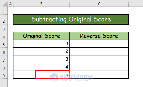
• Find the highest value from the original score.
• In our example, the highest value is 5.
• Add 1 with the highest value for subtraction.
• The value will be 5+1 = 6.

Step 2:

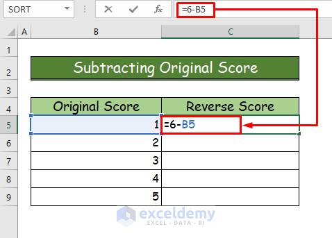
• Add the following formula in cell C5.

• Subtract each original score from 6 to get the reverse score.

Step 3:

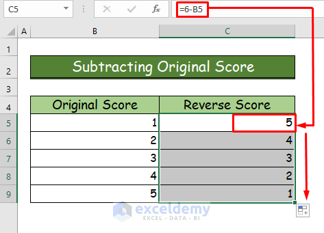
• Press Enter to see the reverse score for 1 which will be 5.
• Use AutoFill to find the reverse scores for the following original scores.

Method 2 – Using IF Function to Reverse Score in Excel

Step 1:

• Enter the following formula in cell C5.

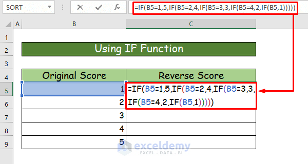
Step 2:

• Press Enter.
• Use the AutoFill feature of Excel to get the reverse scores in all the following cells.

Method 3 – Inserting LOOKUP Function to Reverse Score in Excel

Step 1:

• Select the cell where you want to see the output.
• In our data set, it is cell C5.
• Enter the following formula of the LOOKUP function in the cell.

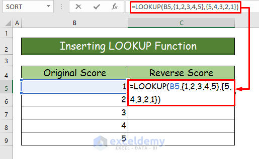
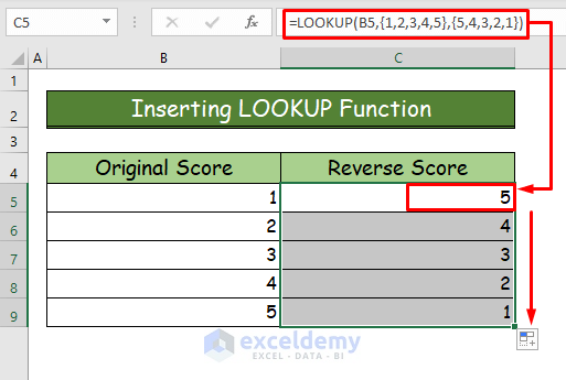
Step 2:

• Press Enter.
• To get the reverse score for the lower cells of the data set use AutoFill tool.

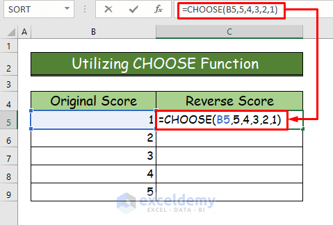
Method 4 – Utilizing CHOOSE Function

Step 1:

• Enter the following formula in cell C5.

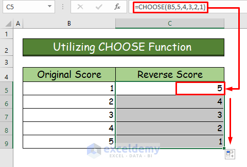
Step 2:

• Press Enter.
• Use AutoFill feature to find out the reverse scores for all the other lower cells.

Download Practice Workbook

<< Go Back to Scoring | Formula List | Learn Excel