Dataset Overview
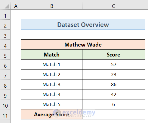
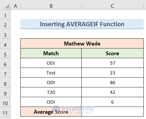
Let’s start by introducing our dataset. We have Mathew Wade as our batsman, and our goal is to calculate his average score for 5 matches. We’ll explore different methods to achieve this using Excel functions.
Method 1 – Using Arithmetic Formula
- Select cell C11.
- Enter the following formula:
=(C6+C7+C8+C9+C10)/5- Press Enter to calculate the average score for Mathew Wade across 5 matches.

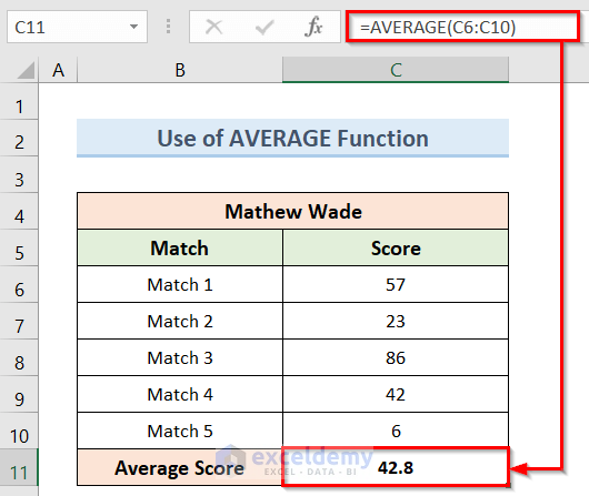
Method 2 – AVERAGE Function
- Select cell C11.
- Enter the formula:
=AVERAGE(C6:C10)- Press Enter to find the direct average of Mathew Wade’s scores.
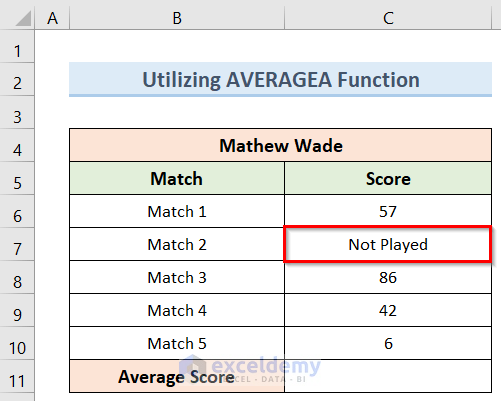
Method 3 – AVERAGEA Function (Handling Text Cells)
To demonstrate how AVERAGEA function works, we have changed the run of Match 2 to Not Played.
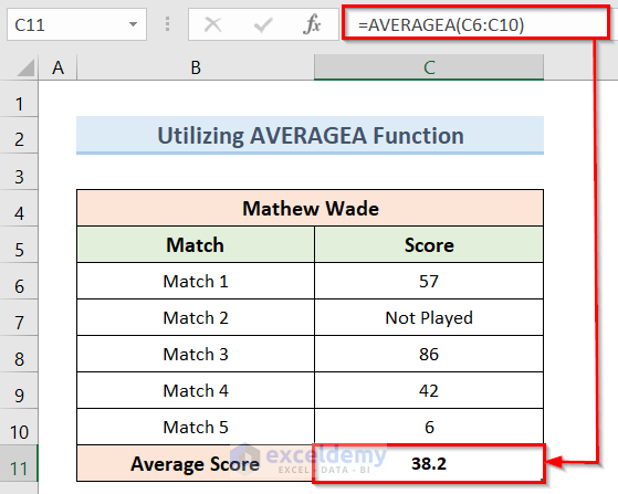
- Select cell C11.
- Insert the formula:
=AVERAGEA(C6:C10)- Press Enter to calculate the average, even if some cells contain text (evaluates text as zero, TRUE as 1, and FALSE as zero).
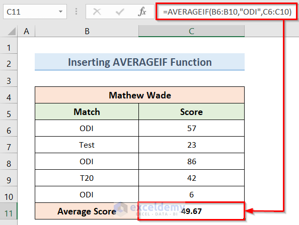
Method 4 – AVERAGEIF Function (Conditional Average)
To demonstrate how the AVERAGEIF function works, we have changed the match types as ODI, Test and T20 in the dataset. Now, our goal is to calculate the average score of Mathew Wade for ODI matches only by using the AVERAGEIF function in Excel.
- Select cell C11.
- Insert the formula:
=AVERAGEIF(B6:B10,"ODI",C6:C10)- Press Enter to find the average score for Mathew Wade in ODI matches.
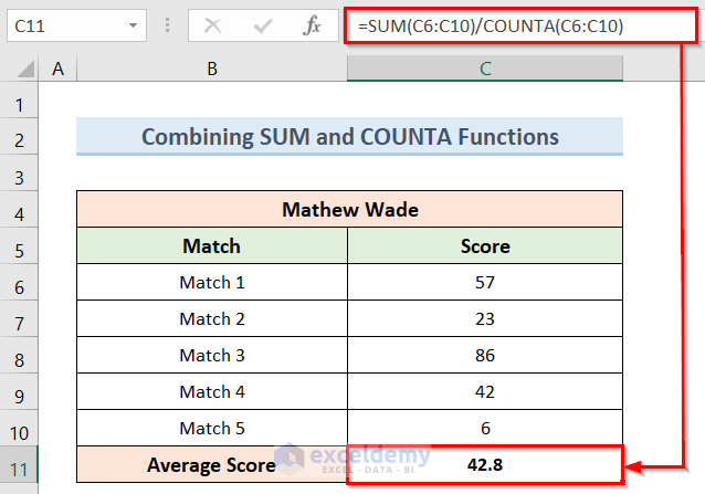
Method 5 – Combining SUM and COUNTA Functions
- Select cell C11.
- Enter this formula:
=SUM(C6:C10)/COUNTA(C6:C10)- Press Enter to calculate the average score by summing the scores and dividing by the count of non-empty cells.
How Does the Formula Work?
- SUM(C6:C10) calculates the sum of Mathew Wade’s scores (from cells C6 to C10).
- COUNTA(C6:C10) counts the number of non-empty cells in the same range.
- The result of the sum is divided by the count to compute the average.
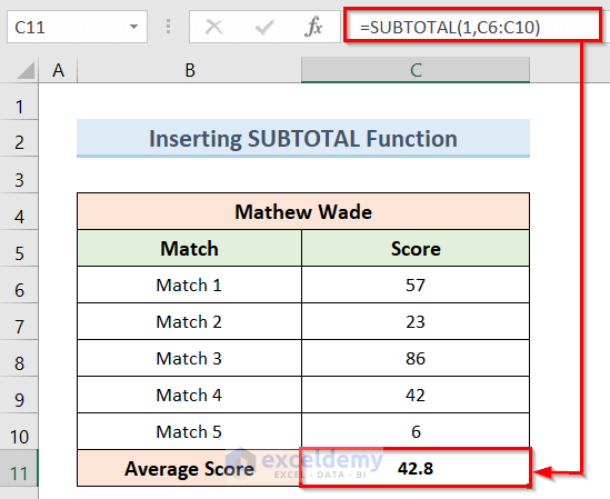
Method 6 – Using the SUBTOTAL Function
The SUBTOTAL function is a powerful tool in Excel. It allows us to perform various calculations within a specified range, while also considering hidden or filtered data. Here’s how to use it to calculate the average score for Mathew Wade across 5 matches:
- Select cell C11.
- Insert the following formula:
=SUBTOTAL(1,C6:C10)- Press Enter to calculate the average of Mathew Wade’s scores.
In the formula, the number 1 corresponds to the AVERAGE function within the SUBTOTAL. This means it will calculate the average of the visible values in the specified range.
Method 7 – Calculating Average Highs and Lows with the AVERAGE and LARGE or SMALL Functions
We can also determine the average of the highest or lowest scores using combinations of AVERAGE with either the LARGE or SMALL function. This approach provides flexibility. Let’s explore both scenarios:
7.1 Calculating Average of 3 Highest Runs
To find the average of Mathew Wade’s highest 3 scores, follow these steps:
- Select cell C11.
- Insert the formula:
=AVERAGE(LARGE(C6:C10,{1,2,3}))- Press Enter to calculate the average of the 3 highest runs.

How Does the Formula Work?
- LARGE(C6:C10, {1, 2, 3}) returns the three largest values from cells C6 to C10.
- The AVERAGE function then computes the average of these three values.
7.2 Calculating Average of 3 Lowest Runs
For the average of Mathew Wade’s lowest 3 scores, follow these steps:
- Select cell C11.
- Enter the formula:
=AVERAGE(SMALL(C6:C10,{1,2,3}))- Press Enter to calculate the average of the 3 lowest runs.
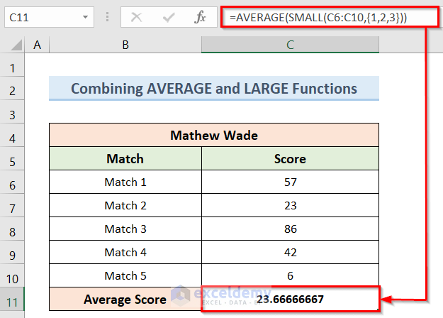
How Does the Formula Work?
- SMALL(C6:C10, {1, 2, 3}) returns the three smallest values from cells C6 to C10.
- The AVERAGE function then computes the average of these three values.
Things to Remember
- If you’re dealing with a large dataset, avoid using the Arithmetic formula (adding individual scores) due to its length.
- When applying conditions, the AVERAGEIF function is ideal.
- For calculating averages based on highest or lowest scores, combining AVERAGE with LARGE or SMALL functions is effective.
Download Practice Workbook
You can download the practice workbook from here:
<< Go Back to Scoring | Formula List | Learn Excel
Get FREE Advanced Excel Exercises with Solutions!

I fully understand this. But I’m trying this without the total of a game. I want to find the average per turn over multiple games. So I got a two-dimentional array with scores of multiple people and I want to find the average for player x. =AVERAGEIF(‘Quirkle scores’!$B$1:$ZZ$1; “*”&E2&”*”;’Quirkle scores’!$B$4:$ZZ$101) This is what I came up with so far. But I haven’t yet found an answer. So I’m looking in B1;ZZ1 for a name in E2. And than I want to average all those columns combined. But with AVERAGEIF it only looks at B4:ZZ4 now instead of B4:ZZ101. Would love to hear another insight.
Dear Wietze,
Thank you for your comment. unfortunately, your question seems unclear to me. If you can provide me with your Excel file and be more specific about your inquiry, I will be able to help you. Please share your Excel file.
Best,
Afia Aziz Kona