How to Create a Balanced Scorecard in Excel (with Detailed Steps)

Step 1 – Assign Factors for the Scorecard Model

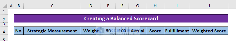
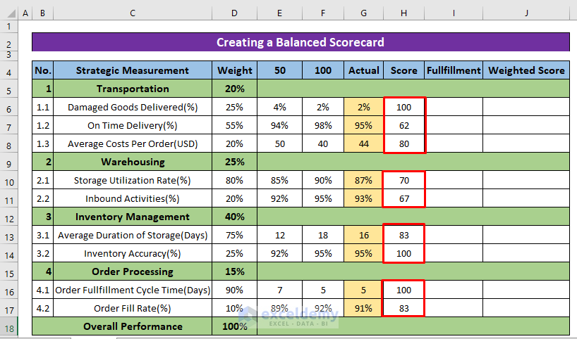
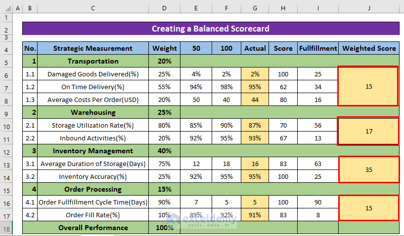
• Assign the parameters which will determine the performance of the company. These are the parameters for this example:

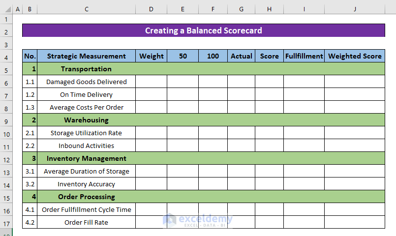
• To assign strategic goals under each of the categories, first define which factors affect performance for each category.
• Add them to the scorecard.

Step 2 – Set Weight to the Scorecard

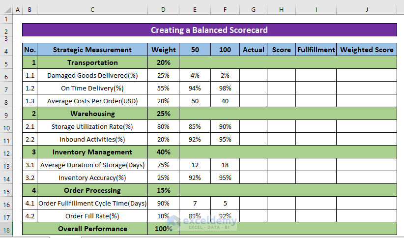
• Set the percentages of the categories (i.e. Weight) that affect the performance of the organization.

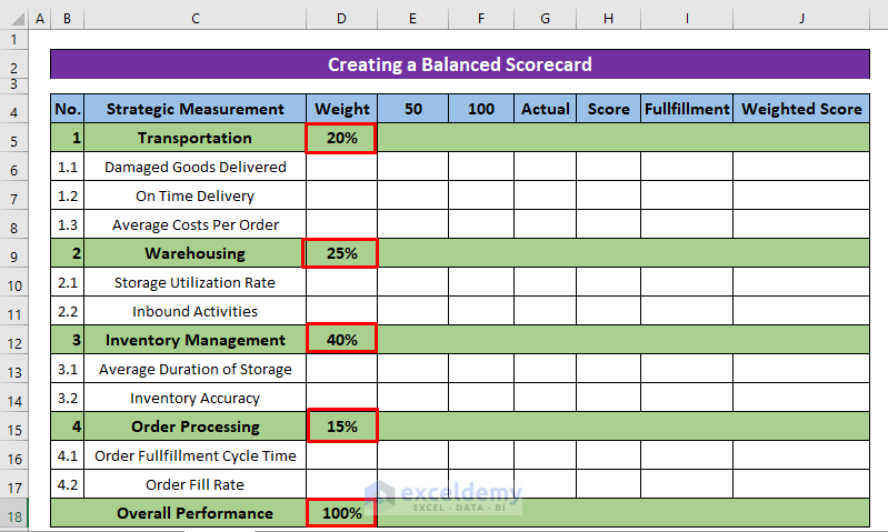
Note: Make sure that the total weight of the categories equals 100%.

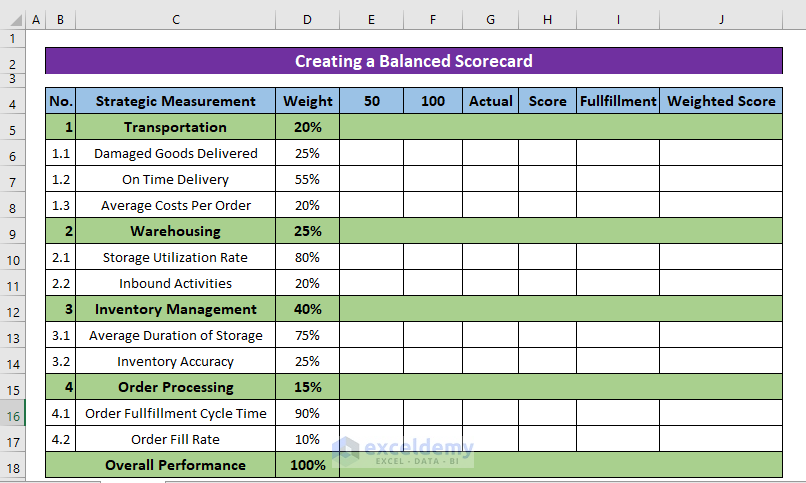
• Assign percentages to the strategic goals under each of the categories. Just like the categories, the subtotal of each of these should equal 100%.

For example, Transportation has 3 factors:

1. Damaged  Goods Delivered (25%)
2. On-Time Delivery (55%)
3. Average Costs Per Order (20%)

The total of these factors is: 25%+55%+20%=100%.

Step 3 – Calculate Score in Model

• The next two column headings (E4 and F4) denote scores for the corresponding inputs. In this example, the score will increase with the decrease of the damaged products.

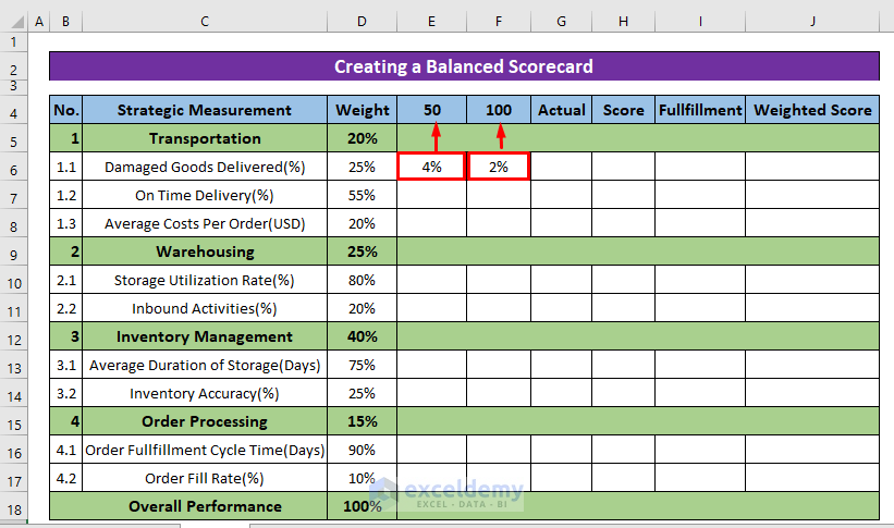
• Assign values for the determined scores (50 and 100) for each of the factors.

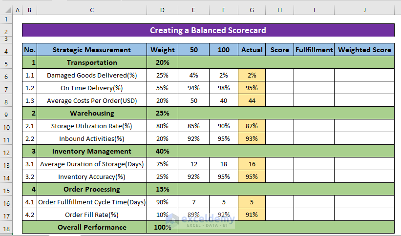
• Input the Actual values under each category.

• Choose the first Actual value (G6) and apply the following formula:

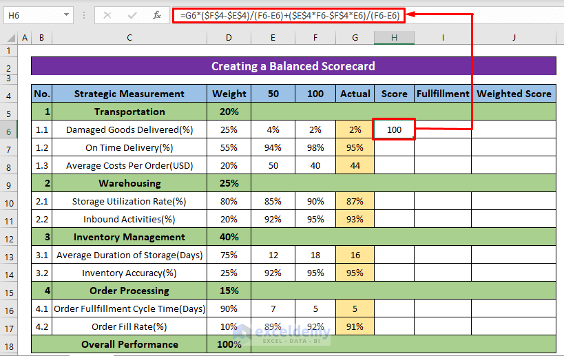
• Use the Autofill Tool to copy the formula to the remaining cells.

Step 4 – Create the Balanced Scorecard

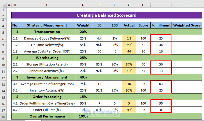
• Apply the following formula to the fulfillment column (I6):

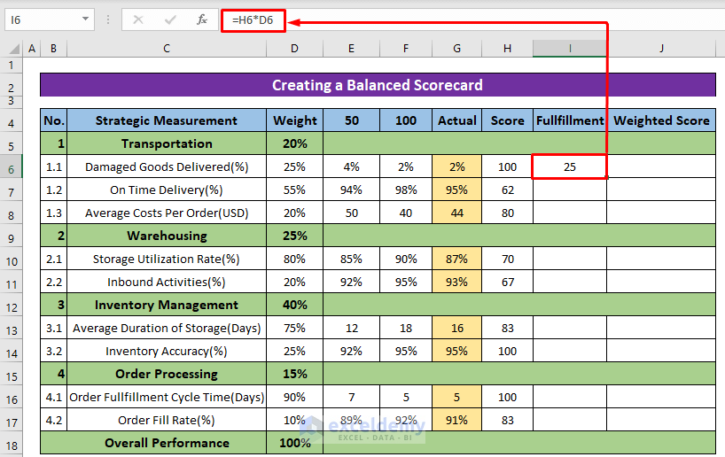
• Use the Autofill Tool to copy the formula to the remaining cells.

• Use the SUM function and the following formula to calculate the weighted score:

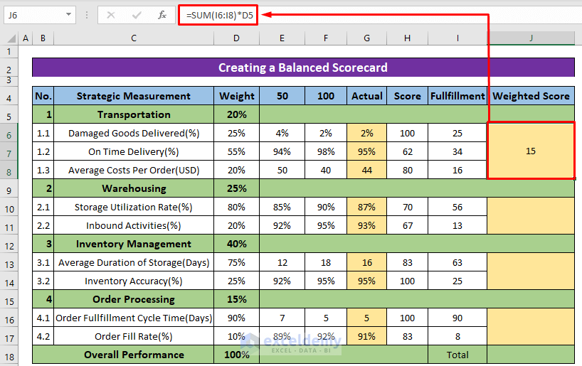
• Use the formula to calculate the Weighted Score for all the other categories.

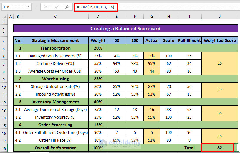
• Calculate the Total Weighed Score with the following formula:

Download Practice Workbook

You can download the practice book below.

<< Go Back to Scoring | Formula List | Learn Excel