This is an overview.
Introduction to the RANK Function in Excel

- Objective:
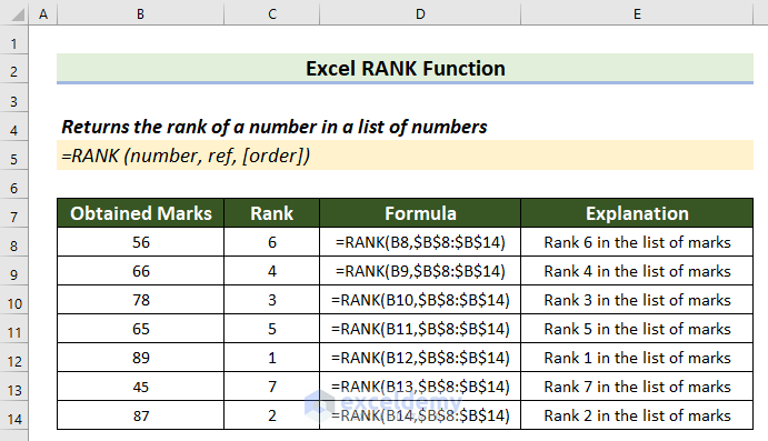
The RANK function returns the position of a given number in a given list of numbers.
- Syntax:
=RANK(number,ref,[order])- Arguments:
| Argument | Required/Optional | Value |
|---|---|---|
| number | Required | The number that you want to rank. |
| ref | Required | It is the reference (an array or a list of numbers) that contains the number. |
| [order] | Optional | The ranking method. 0 is used for descending order, and 1 for ascending order. |
- Return Parameter:
It returns a rank number.
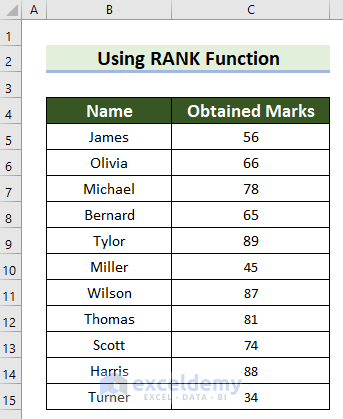
The dataset contains students’ names and their marks.
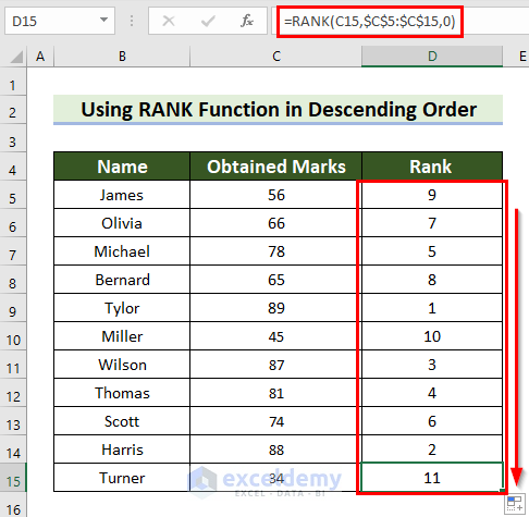
Example 1 – Use the RANK Function in Descending Order
Steps:
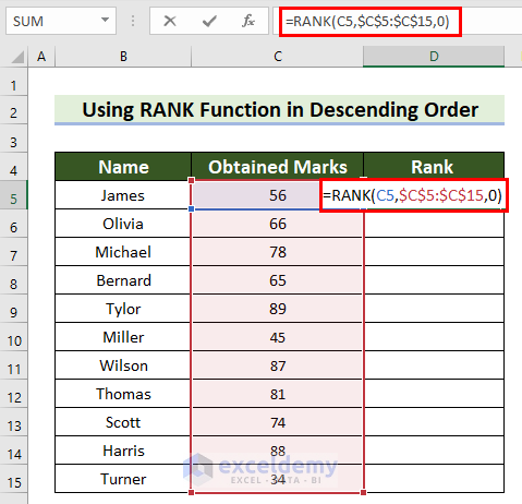
- Select a cell to see the rank. Here, D5.
- Enter the following formula.
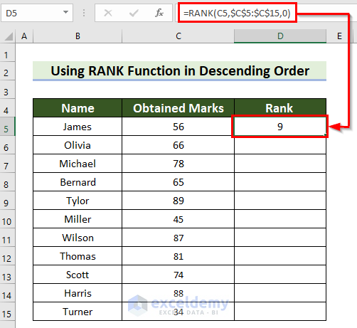
=RANK(C5,$C$5:$C$15,0)- Press Enter to see the result.
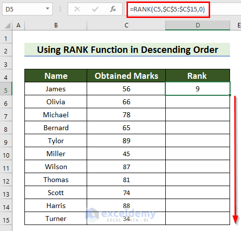
- Drag the Fill Handle down to copy the formula.
- This is the output.
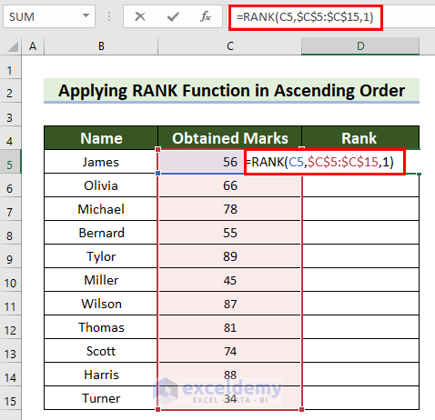
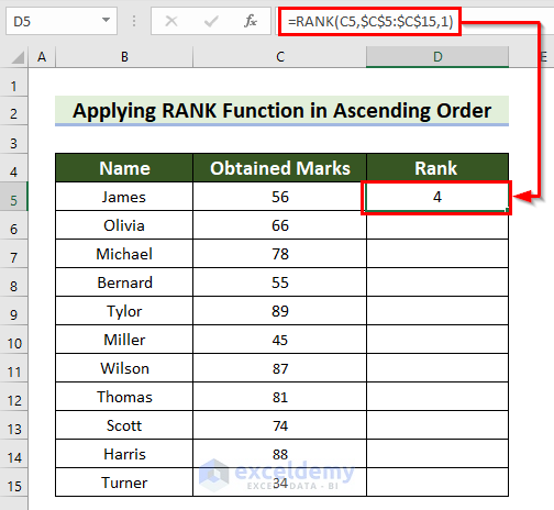
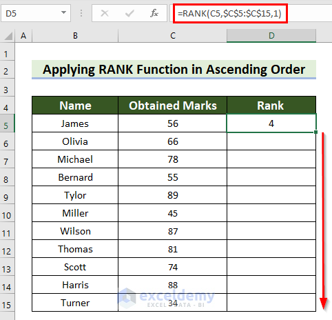
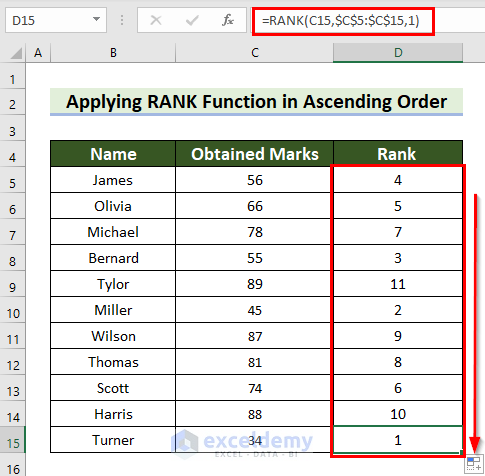
Example 2 – Apply the RANK Function in Ascending Order in Excel
Steps:
- Select a cell to see the rank. Here, D5.
- Enter the following formula.
=RANK(C5,$C$5:$C$15,1)- Press Enter to see the result.
- Drag the Fill Handle down to copy the formula.
- This is the output.
Read More: Ranking Data in Excel with Sorting
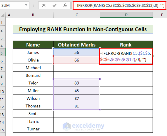
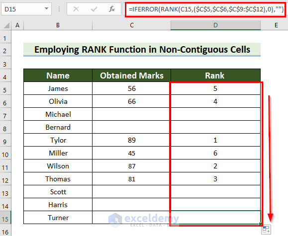
Example 3 – Apply the RANK Function in Non-Contiguous Cells
Steps:
- Select a cell to see the rank.
- Enter the following formula in the selected cell.
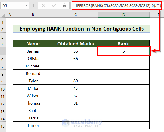
=IFERROR(RANK(C5,($C$5,$C$6,$C$9:$C$12),0),"")- Press Enter to see the result.
Formula Breakdown
- RANK(C5,($C$5,$C$6,$C$9:$C$12),0): l C5 is the number, ($C$5,$C$6,$C$9:$C$12) is the ref, and 0 is the order. The formula returns the rank of C5 in the ref in descending order. If it does not find the number in the ref range, it returns an error.
- IFERROR(RANK(C5,($C$5,$C$6,$C$9:$C$12),0),””): the IFERROR function returns an empty string if it finds an error. Otherwise, it returns the rank.
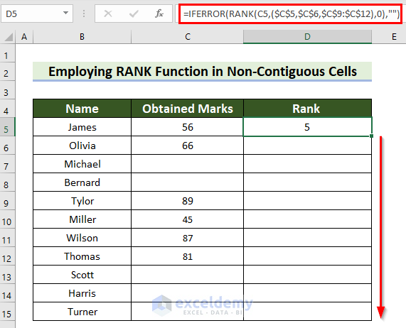
- Drag the Fill Handle down to copy the formula.
- This is the output.
Read More: How to Stack Rank Employees in Excel
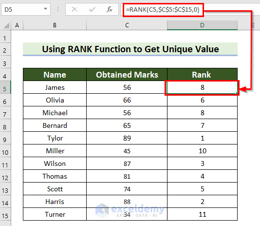
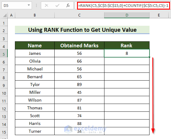
Example 4 – Get a Unique Value Using the Excel RANK Function
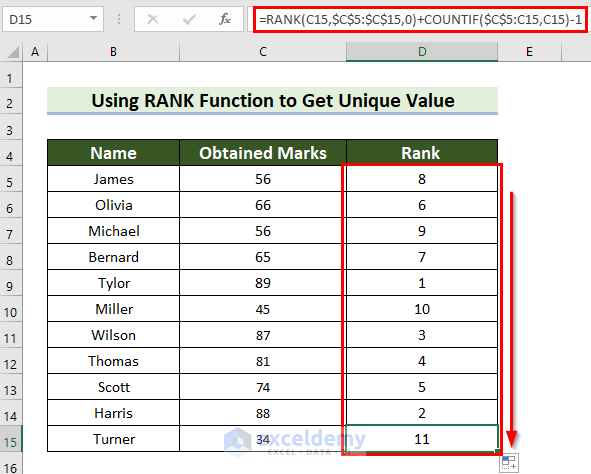
If two students get the same marks, you will find duplicate ranks.
Steps:
- Select a cell to see the rank.
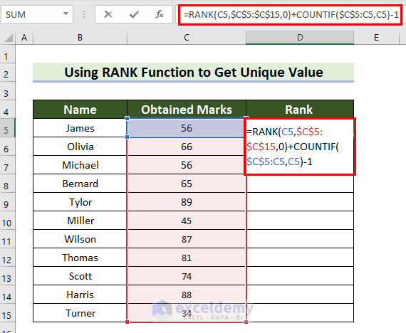
- Enter the following formula in the selected cell.
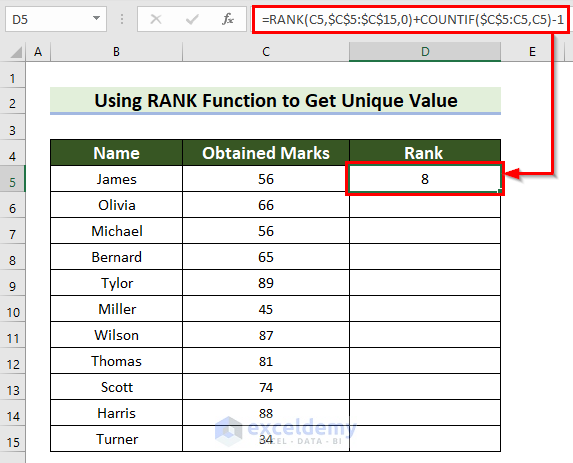
=RANK(C5,$C$5:$C$15,0)+COUNTIF($C$5:C5,C5)-1- Press Enter to see the result.
Formula Breakdown
- RANK(C5,$C$5:$C$15,0): C5 is the number, C5:C15 is the ref, and 0 is the order. The formula returns the rank of the value in C5 among C5:C15 in descending order.
- COUNTIF($C$5:C5,C5): In the COUNTIF function, $C$5:C5 is the range and C5 is the criteria. The formula returns the number of cells in the range that match the criteria.
- RANK(C5,$C$5:$C$15,0)+COUNTIF($C$5:C5,C5)-1: this formula sums the results and subtracts 1.
- Drag the Fill Handle down to copy the formula.
- This is the output.
Read More: Excel Formula to Rank with Duplicates
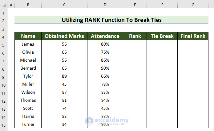
Example 5 – Utilize the RANK Function to Break Ties in Excel
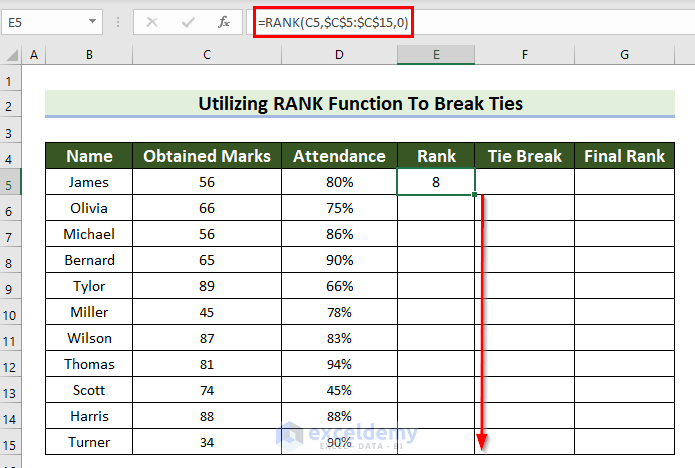
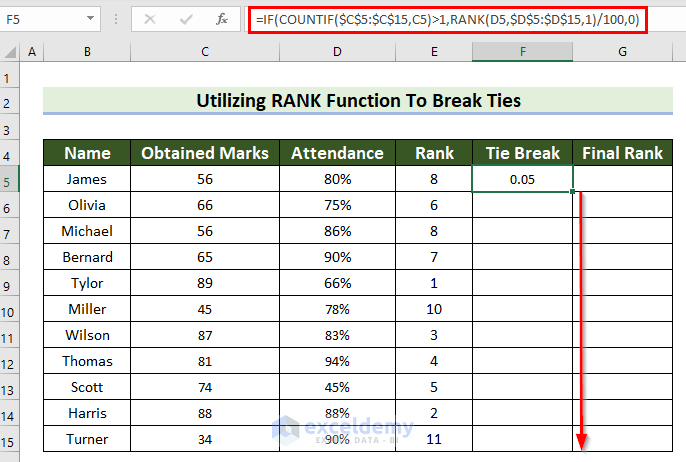
The percentage of Attendance is given for each student. The dataset contains both Obtained Marks and Attendance.
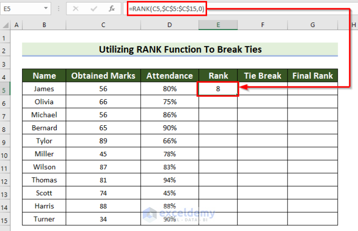
Steps:
- Select a cell to see the rank.
- Enter the following formula in the selected cell.
=RANK(C5,$C$5:$C$15,0)- Press Enter to see the rank.
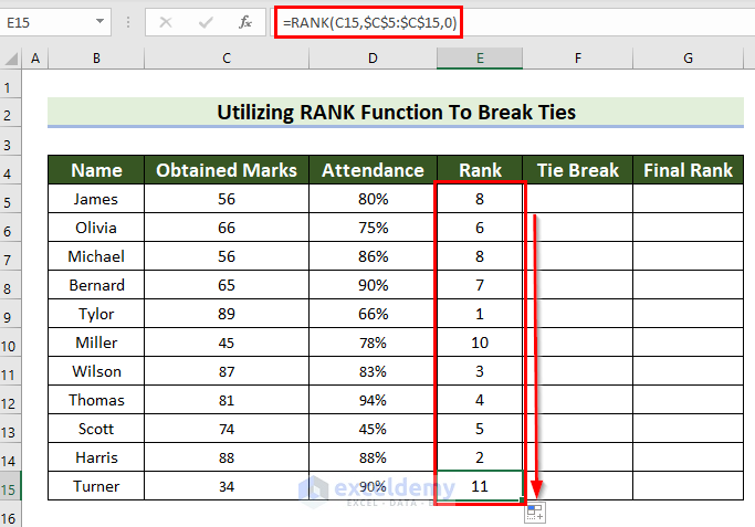
- Drag the Fill Handle down to copy the formula to the other cells.
- This is the output.
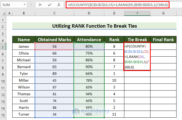
- Select a cell to see the Tie Break. Here, F5.
- Enter the following formula.
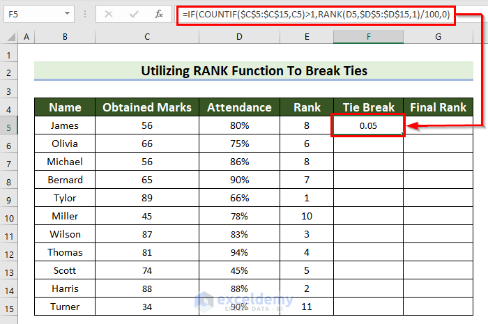
=IF(COUNTIF($C$5:$C$15,C5)>1,RANK(D5,$D$5:$D$15,1)/100,0)- Press Enter to see the result.
Formula Breakdown
- COUNTIF($C$5:$C$15,C5): C5:C15 is the range and C5 is the criteria. The formula returns the number of cells in the selected range that match the given criteria.
- RANK(D5,$D$5:$D$15,1): D5 is the number, D5:D15 is the ref, and 1 is the order. The formula ranks the values in ascending order.
- RANK(D5,$D$5:$D$15,1)/100: the result is divided by 100.
- IF(COUNTIF($C$5:$C$15,C5)>1,RANK(D5,$D$5:$D$15,1)/100,0): the IF function checks if the value returned by the COUNTIF is greater than 1. If the logical_test is True, it is inserted in the RANK function. Otherwise, it returns 0.
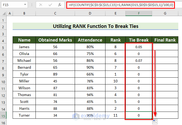
- Drag the Fill Handle down to copy the formula to the other cells.
- This is the output.
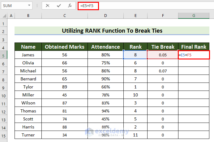
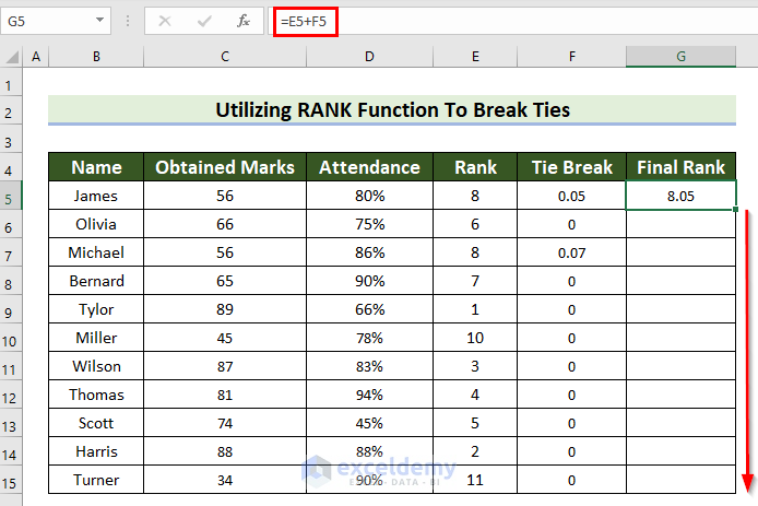
To see the Final Rank from the Rank and the Tie Break:
- Select G5.
- Enter the following formula.
=E5+F5- Press Enter to see the result.
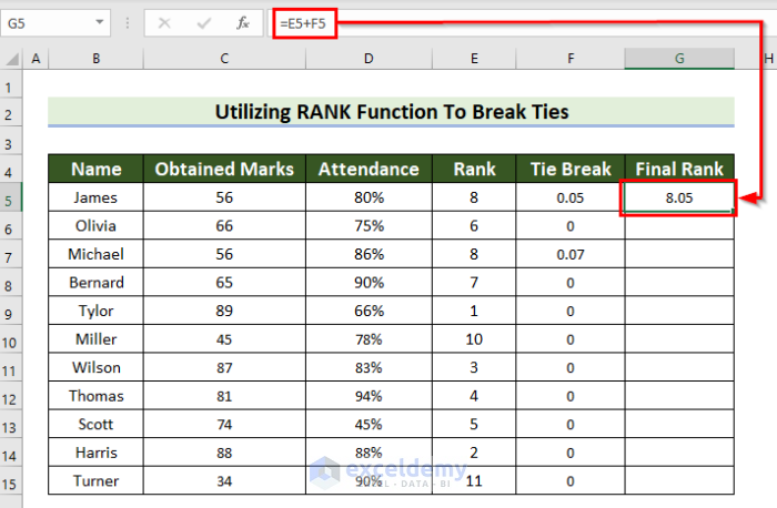
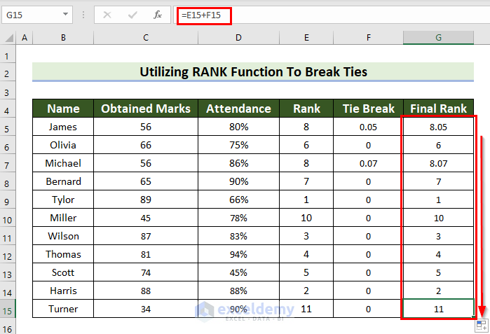
- Drag the Fill Handle down to copy the formula to the other cells.
- This is the output.
Read More: How to Rank with Ties in Excel
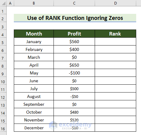
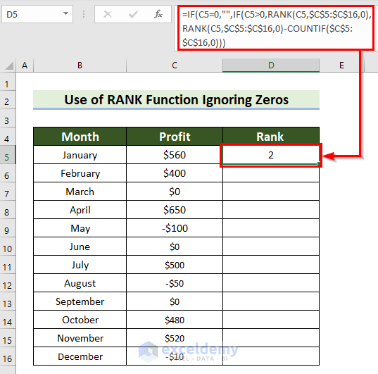
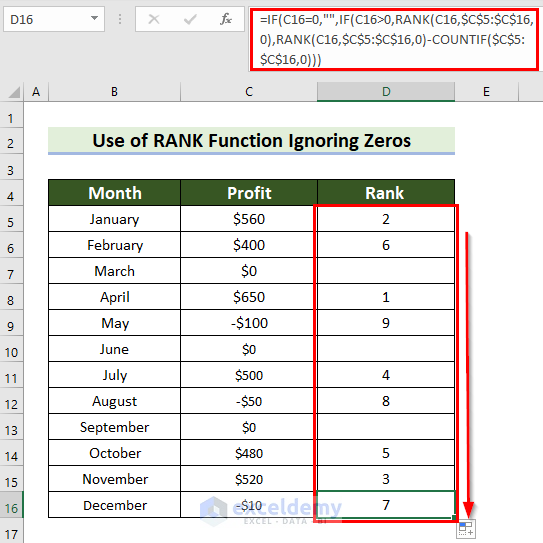
Example 6 – Apply the RANK Function Ignoring Zeros in Excel
Steps:
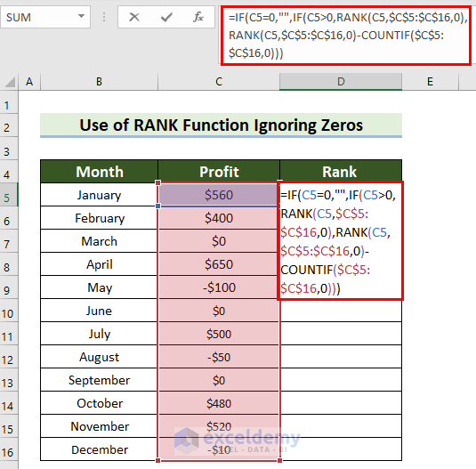
- Select a cell to see the rank.
- Enter the following formula in the selected cell.
=IF(C5=0,"",IF(C5>0,RANK(C5,$C$5:$C$16,0),RANK(C5,$C$5:$C$16,0)-COUNTIF($C$5:$C$16,0)))- Press Enter to see the result.
Formula Breakdown
- RANK(C5,$C$5:$C$16,0): returns the Rank of C5 in C5:C15 in descending order.
- COUNTIF($C$5:$C$16,0): C5:C15 is the range and 0 is the criteria. The formula will return the number of cells that match the criteria.
- RANK(C5,$C$5:$C$16,0)-COUNTIF($C$5:$C$16,0): subtracts the result returned by the COUNTIF function from the result returned by the RANK function.
- IF(C5>0,RANK(C5,$C$5:$C$16,0),RANK(C5,$C$5:$C$16,0)-COUNTIF($C$5:$C$16,0)): checks if the value in C5 is greater than 0. If the logical_test is True, it returns the result from the RANK function. Otherwise, it returns the result from the RANK and the COUNTIF functions.
- IF(C5=0,””,IF(C5>0,RANK(C5,$C$5:$C$16,0),RANK(C5,$C$5:$C$16,0)-COUNTIF($C$5:$C$16,0))): checks if the value in cell C5 is 0. If the logical_test is True, the formula returns an empty string. Otherwise, it moves to the second IF function.
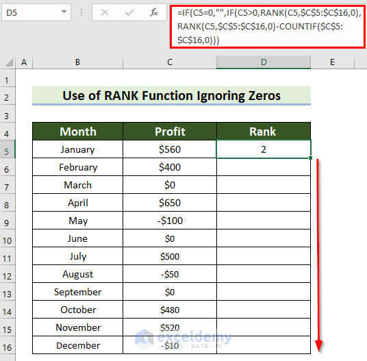
- Drag the Fill Handle down to copy the formula to the other cells.
- This is the output.
Read More: Ranking Based on Multiple Criteria in Excel
Common Error While Using the RANK Function in Excel
#N/A error occurs with the RANK function when the number that you want to rank is not available in the reference.
Things to Remember
- If you omit the order (it is an optional argument), the RANK function will sort automatically in descending order.
Download Practice Workbook
Download the practice workbook here.
Excel RANK Function: Knowledge Hub
<< Go Back to Excel Functions | Learn Excel
Get FREE Advanced Excel Exercises with Solutions!