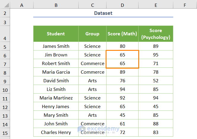
The sample dataset contains student scores in Math and Psychology as well as each student’s group. We’ll rank the students according to the scores.
Method 1 – Using RANK.EQ and COUNTIFS Functions
- Use the following formula:
=RANK.EQ($C5,$C$5:$C$15)+COUNTIFS($C$5:$C$15,$C5,$D$5:$D$15,">"&$D5)
The RANK.EQ function returns the rank number from the C5:C15 cell range based on the C5 cell. It provides the same rank for the duplicate scores (e.g. rank number is 7 for C6, C7, and C12 cells). The COUNTIFS function is assigned in descending order (“>”&$D5) to count duplicate scores. The function returns 1 for the C7 cell and 2 for the C12 cell. When you sum the two outputs, you’ll get the unique rank number for all students.
![]()
- Hit Enter and use the Fill Handle tool.
![]()
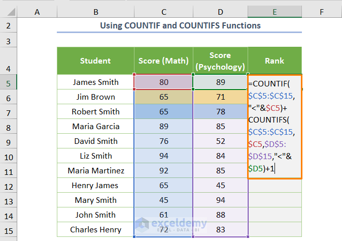
Method 2 – Ranking Based on Multiple Criteria Using COUNTIF and COUNTIFS Functions
- Use the following formula:
=COUNTIF($C$5:$C$15,"<"&$C5)+COUNTIFS($C$5:$C$15,$C5,$D$5:$D$15,"<"&$D5)+1
We want to rank the scores in ascending order (“<“&$D5). The COUNTIF function counts the number of cells in column D with values greater than the corresponding cell (like C5 for James Smith, C6 for Jim Brown, and so on). We then add 1 to make sure the rankings start from 1.
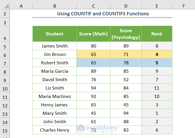
- Here’s the output.
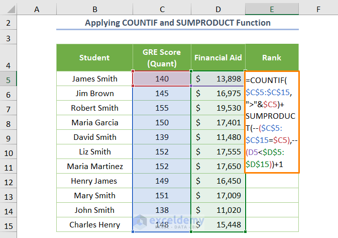
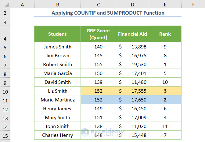
Method 3 – Applying RANK and SUMPRODUCT Functions
In the following dataset, we’ll rank based on the GRE Score (Quant) and Financial Aid.
![]()
- Insert the following formula in E5 and AutoFill through the column:
=RANK(C5,$C$5:$C$15)+SUMPRODUCT(--($C$5:$C$15=$C5),--(D5<$D$5:$D$15))
⧬ Formula Explanation:
- The RANK function returns the rank number from the $C$5:$C$15 cell range based on the C5 cell with the duplicates value in the C10 and C11 cells (the rank number is 2).
- The SUMPRODUCT function finds 0 in case of no tied values. But it returns 1 for the C10 cell.
- The (—) operator is used to return 1 instead of getting TRUE and 0 for FALSE.
![]()
Here are the results.
![]()
- Here’s an alternative formula you can use:
=COUNTIF($C$5:$C$15,">"&$C5)+SUMPRODUCT(--($C$5:$C$15=$C5),--(D5<$D$5:$D$15))+1
You’ll get the same output.
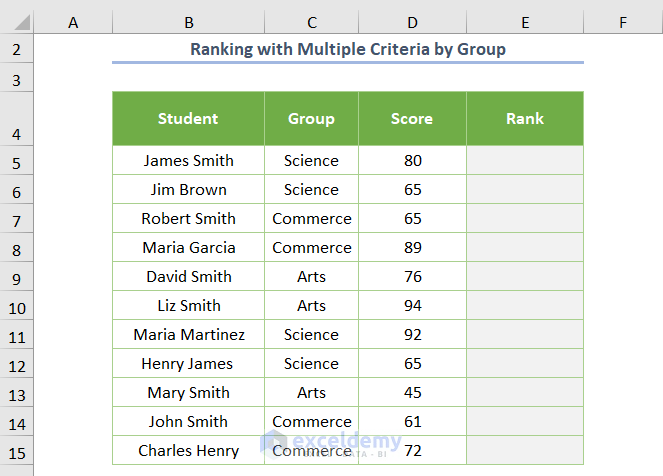
Method 4 – Ranking with Multiple Criteria by Group
What if you have some common Groups in your dataset? For example, the Science group covers C5:C6 and C11:C12 cells.
Case 4.1 – Using the COUNTIFS Function
- Use the following formula and AutoFill through the column.
=COUNTIFS($C$5:$C$15,C5,$D$5:$D$15,">"&D5)+1
⧬ Formula Explanation:
- COUNTIFS($C$5:$C$15,C5) returns 4 as there are 4 cells that contain Science (C5).
- The COUNTIFS($C$5:$C$15,C5,$D$5:$D$15,”>”&D5) syntax returns 0 for the highest scores (e.g. for the E6 cell).
- We’re adding 1 to all rankings.

Read More: How to Rank Within Group in Excel
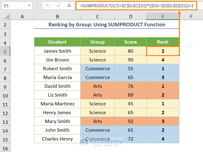
Case 4.2 – Using SUMPRODUCT Function
- Use the following formula:
=SUMPRODUCT((C5=$C$5:$C$15)*($D5<$D$5:$D$15))+1
⧬ Formula Explanation:
- SUMPRODUCT((C5=$C$5:$C$15) returns 0.
- SUMPRODUCT((C5=$C$5:$C$15)*($D5<$D$5:$D$15)) finds 2. But the SUMPRODUCT function returns 0 for E7 cell as it is the smallest score. We added 1 to make a more readable list.
- The formula scores in ascending order, giving 1 to the lowest-scoring student within their group.
Download the Practice Workbook
Related Articles
- How to Rank with Ties in Excel
- How to Calculate the Top 10 Percent in Excel
- How to Rank in Excel Highest to Lowest
- Rank IF Formula in Excel
- Ranking Data in Excel with Sorting
- Excel Formula to Rank with Duplicates
<< Go Back to Excel RANK Function | Excel Functions | Learn Excel
Get FREE Advanced Excel Exercises with Solutions!

I need your support to find a formula for aging stock to put a value to a range of time based on the remaining quantity and aging from invoiced quantity
Hi NGÂN,
The solution you want will require a combination of some functions like TODAY, COUNTIF, VLOOKUP, etc. Here is a post on our website that will help you.
https://www.exceldemy.com/stock-ageing-analysis-formula-in-excel/
We have several posts related to this topic too.
https://www.exceldemy.com/make-inventory-aging-report-in-excel/
https://www.exceldemy.com/excel-ageing-formula-for-30-60-90-days/
https://www.exceldemy.com/aging-of-accounts-receivable-in-excel/
I hope these articles will help get your job done. If not, please remember that we are just a text away!!
Thank you. Have a good day.
Thanks for providing the guide. How do you rank without duplicates in the case of 4. Ranking with Multiple Criteria by Group? So instead of having duplicate ranks, I want to avoid them without skipping any number. Thanks in advance
Greetings Edward,
Thanks a lot for your Question in our blog post. Now the issue you have is a little bit unclear to me. Can you provide a sample output manually which will contain your desired result? In that way, your problem be more clear to us and in turn it will help us to resolve your problem.
How would you rank with multiple criteria and duplicates? In the initial example above, you see Jim Brown and Henry James with Science and 65 scores. How would you rank and not repeat numbers?
Thank you.
Hello GUILLERMO ALCALA,
Thank you for your comment. In the initial example, Jim Brown, Robert Smith, and Henry James scored 65 in Science. So if you rank them according to the score of Science, you will get repeated ranks. But, as you can see, these 3 students got different scores in Psychology. So, we have ranked them according to the E column (Psychology). Hence, the rank is not repeated, and they got different ranks according to Psychology score.
Regards
Mahfuza Anika Era
Exceldemy
I am looking for a ranking formula that will rank salesmen by region based on number of units sold and then (in the case of ties) by total sales amount. I need unique rankings so there are no duplicates. Any help you can provide is greatly appreciated. I have tried this so many ways and never getting the desired outcome.
Hello Denise Sano
Thanks for visiting our blog and leaving an exciting comment. You want to rank salespeople by region based on number of units sold and then (in the case of ties) by total sales amount. However, developing such a formula using Excel’s built-in function would be time-consuming.
So, I have developed an Excel VBA sub-procedure to help you overcome your situation.
Follow these steps:
As a result, you get the intended rank like the following GIF.
I have attached the solution workbook for better understanding. Hopefully, the idea will help; good luck.
DOWNLOAD SOLUTION WORKBOOK
Regards
Lutfor Rahman Shimanto
Excel & VBA Developer
ExcelDemy