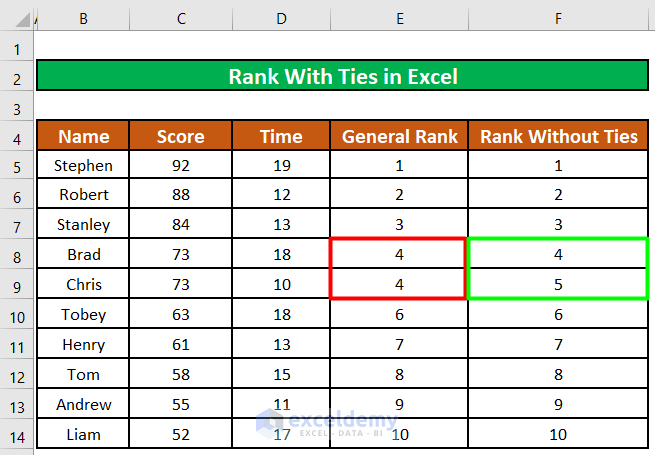
Consider the worksheet below, which contains the results of a sporting contest. We have the Names of the participants, their Scores, their Times, and their Ranks based on the performance. Chris and Brad are tied, as they achieved the same score. The image below shows the General Ranking with the tie reflected, and also the Rank without Ties. We will use this Excel worksheet to demonstrate how to rank with ties in Excel.
Method 1 – Ranking First Value in a Tie the Superior Position
Let’s first rank the data with only one criterion, the Scores in the contest.
Steps:
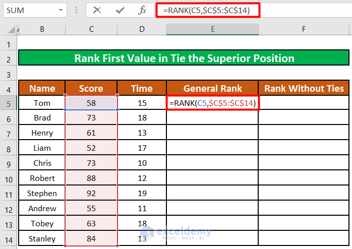
- Enter the formula below in cell E5:
=RANK(C5,$C$5:$C$14)Formula Explanation:
- The RANK function takes two arguments; the first is the value of cell C5 while the second is the absolute range $C$5:$C$14.
- The function will try to determine the rank or order of the cell value C5 in the absolute range $C$5:$C$14.
- Press ENTER
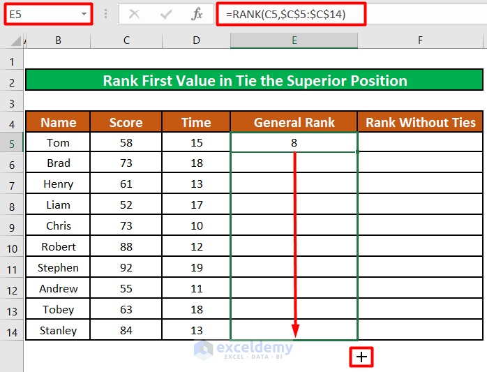
The participant in the first row (C5) has been ranked as 8th.
- Drag the fill handle of cell E5 to apply the formula to the rest of the cells under General Rank.
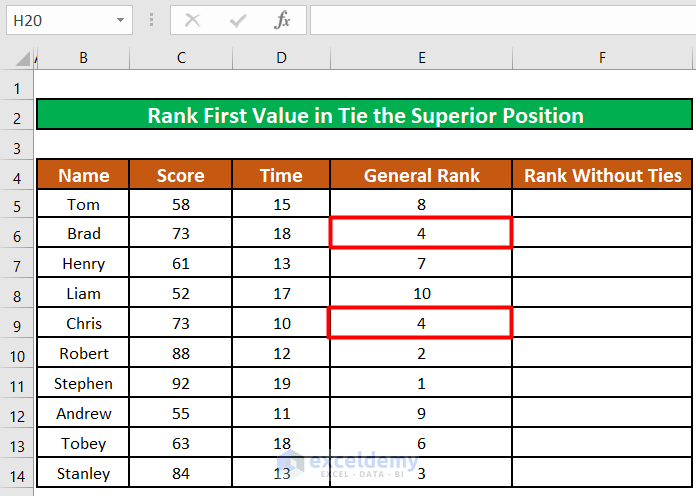
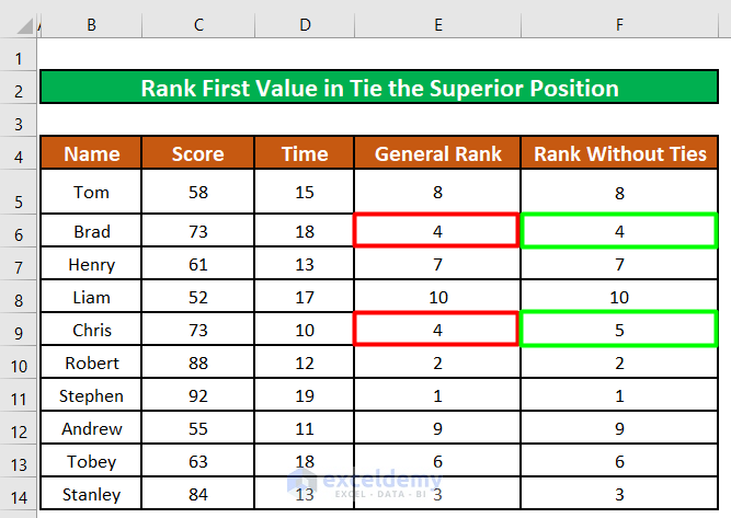
All the participants are ranked, and 2 participants named Brad (cell B6) and Chris (cell B9) are ranked in the same position (Rank 4th).
- Enter the formula below in cell F5 to break the tie in the rank.
=RANK(C5,$C$5:$C$14)+COUNTIF(C$5:C5,C5)-1Formula Explanation:
- COUNTIF function takes the expanding range C$5:C5 as the first argument and the cell value C5 as the second argument. It will try to find out how many times the value in C5 appears in the expanding range.
- The value returned by the COUNTIF function will then be added to the value returned by the RANK function and 1 will be subtracted.
- When this formula is applied to the first tied rank (cell E6), the COUNTIF function will return 1 as rank 4 appears only once to that point.
- As the value (1) returned by the COUNTIF function will be added to the value returned by the RANK function and 1 will be subtracted, the RANK of the participant Brad will remain unchanged.
- The value returned by the RANK function = 4
- The value returned by the COUNTIF function = 1
- Value to be subtracted = 1
- So, the formula will return the value = 4 + 1 – 1 = 4
- In the case of the second tied rank (cell E9), the COUNTIF function will return 2, as rank 4 appears twice to that point.
- As the value (2) returned by the COUNTIF function will be added to the value returned by the RANK function while 1 will be subtracted, the RANK of the participant Chris will be increased to 5.
- The value returned by the RANK function = 4
- The value returned by the COUNTIF function = 2
- Value to be subtracted = 1
- So, the formula will return the value = 4 + 2 – 1 = 5
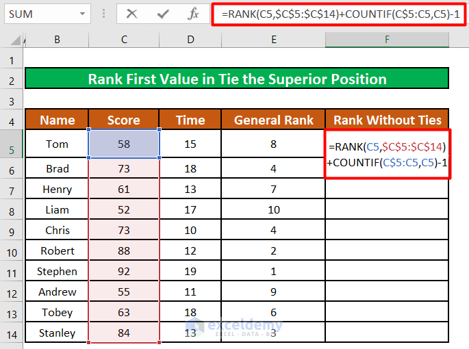
- Press ENTER.
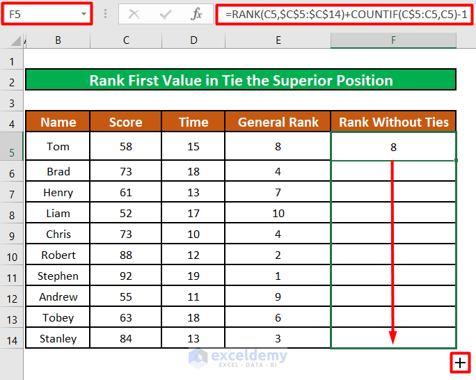
Cell F5 now shows 8 as the rank of the participant in cell B5.
- Drag the fill handle of cell F5 to apply the formula to the rest of the cells.
The rank of the Brad remains 4th while the following participant Chris is now ranked 5th.
Read More: Rank IF Formula in Excel
Method 2 – Using Two COUNTIF Functions Together to Break the Tie in a Rank
For this example, we will rank the participants based on the Time they needed to complete the task.
Steps:
- Rank all the participants based Time they needed to complete the task as above.
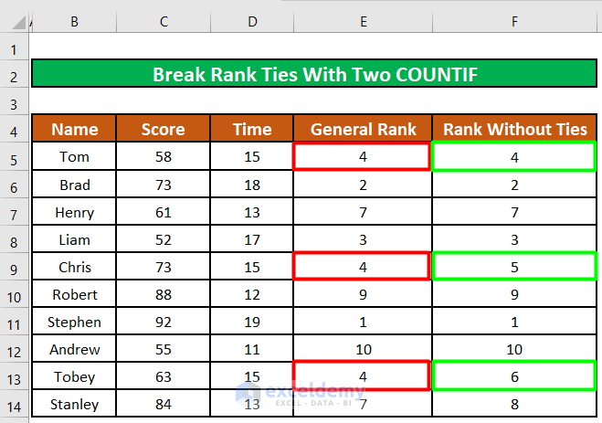
After ranking all the participants, 3 participants named Brad (cell B6), Chris (cell B9), and Tobey (cell B13) are ranked in the same position (Rank 4th).
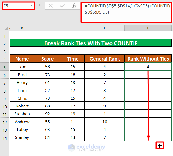
- Enter the below formula in cell E5:
=COUNTIF($D$5:$D$14,">"&$D5)+COUNTIF($D$5:D5,D5)Formula Explanation:
- The first COUNTIF function takes the absolute range $D$5:$D$14 as the first argument and the value of cell D5 as the second argument. It uses the greater than (>) sign to determine how many values in $D$5:$D$14 are greater than D5.
- The second COUNTIF function takes the expanding range D$5:D5 as the first argument and the value of cell D5 as the second argument. It will try to find out how many times the value in D5 appears in the expanding range.
- The two values returned from the two COUNTIF functions will then be summed.
- The first COUNTIF function is basically the RANK function but it will return a value one (1) less than the value returned by RANK, because it will only return the number of those values greater than the cell D5 while the RANK function will return one (1) more than that number.
- The second COUNTIF function is similar to the COUNTIF function used in Method 1. So the sum of the values will be similar to the value returned by the formula in Method 1.
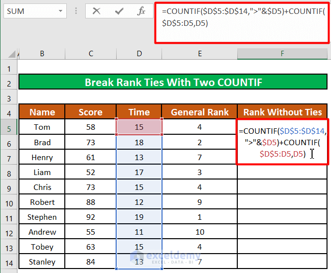
- Press ENTER.
Cell F5 displays 4 as the rank of the participant in cell B5.
- Drag the fill handle of cell F5 to apply the formula to the rest of the cells.
The ranks of all the participants remain unchanged except for the three participants who shared the same rank before (Rank 4th).
Brad remains in 4th position, while the following participant Chris is now ranked 5th and the last participant Tobey holds the 6th position.
Method 3 – Use a Second Criteria to Break the Tie in a Rank
Steps:
- Enter the below formula in cell F5:
=IF(COUNTIF($C$5:$C$14,C5)>1,RANK(D5,$D$5:$D$14,1)/100,0)Formula Breakdown:
- The first argument or the logical test for the IF function is COUNTIF($C$5:$C$14,C5)>1. So, the IF function will determine if the number of appearances of the cell value in C5 in the absolute range $C$5:$C$14 is greater than 1.
- The second argument for the IF function is what it will return if the logical test is TRUE. We have inserted RANK(D5,$D$5:$D$14,1)/100 as the second argument. So, the RANK function will determine the rank of the participants based on the Time they took to complete the task. The first argument for the RANK function is Time (D5), the second is the absolute range of the Time column $D$5:$D$14, and the last argument is 1 which tells the RANK function to rank the participants in ascending order. We will divide the return value of the RANK function by 100 to get a decimal value less than 1.
- The third argument for the IF function is what it will return if the logical test is FALSE. We have inserted zero (0).
- Every value in the absolute range $C$5:$C$14 or each value in the Score column except for the value in cells B6 and B9 (Score 73) only appears once. So, the COUNTIF function will return 1 as the number of the appearance of the cell value in C5. Hence, the Logical Test of the IF function will return FALSE and the function itself will return 0.
- But in the case of cells B6 and B9 (Score 73), the number of appearances is 2.
- Therefore the Logical Test of the IF function will return TRUE and the function itself will return a decimal number, which is the return value of the RANK function (Based on the Time column) divided by 100. The rank for the two cell values will be different this time, which will act as the tie-breaker.
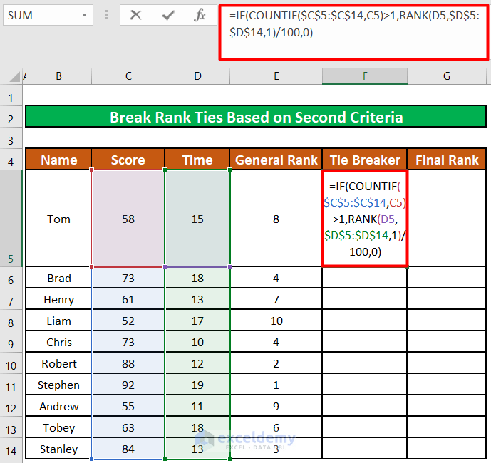
- Press ENTER.
Cell F5 shows the value zero(0).
- Drag the fill handle of cell F5 to apply the formula to the rest of the cells.
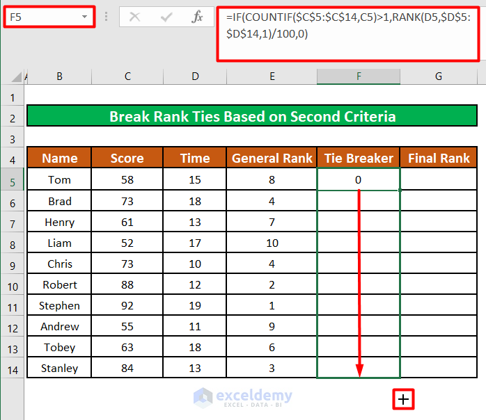
The formula populates each cell in the Tie Breaker column with zero (0), except the two cells that shared the same rank (Rank 4th).
The preceding cell has the value of 0.08 while the following cell has the value of 0.01.
- Enter the below formula in cell G5:
=SUM(E5,F5)Formula Breakdown:
- The SUM function will sum the existing rank value (E5) and the second rank value based on the Time (F5) to determine the Final Rank.
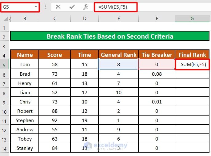
- Press ENTER.
The Final Rank for the first participant is returned.
- Drag the fill handle of cell G5 to apply the formula to the rest of the cells.
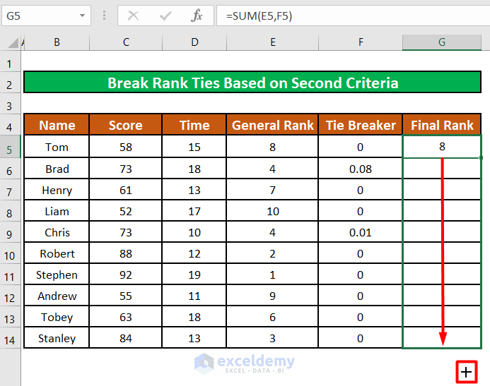
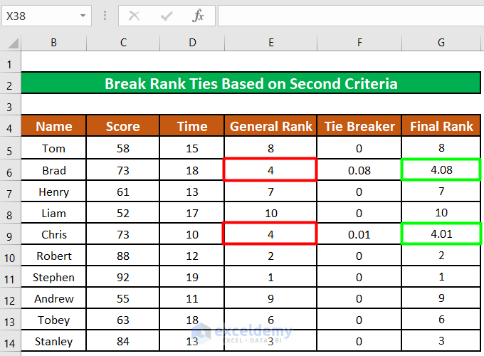
The separate ranks for the two participants in the Tie Breaker column are added to the existing ranks.
Read More: Ranking Based on Multiple Criteria in Excel
Method 4 – Split the Available Winnings For a Ranked Tied Between the Rank Holders
Sometimes when distributing the prize or points in a competition, we might not want to break the tie in a specific rank. Instead, we might want to distribute the prize or points specified for that rank among all the tied participants. For example, suppose we have specified the prize for each rank. We will now split the prizes specified for the 4th, 5th, and 6th positions equally between the 3 participants holding the same 4th position.
Steps:
- Enter the below formula in the cell:
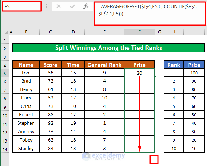
=AVERAGE(OFFSET($I$4,E5,0, COUNTIF($E$5:$E$14,E5)))Formula Breakdown:
- OFFSET function takes 4 arguments. The first is the cell reference. In this case, it is the absolute reference to cell I4 ($I$4). So the reference will not change when we drag the fill handle.
- The second argument is the number of rows down from the cell specified in the first argument (I4). In this example, it is the respective value in the same row of the General Rank (E5:E14). So, for the first cell (cell F5), it is 9 (cell E5). OFFSET will refer to the cell in the Prize column (Column I) that is 9 rows down from cell I4. That cell is I13 and it refers to the prize specified for rank 9. As we drag the fill handle to apply the formula to different cells in this column (Column F), the OFFSET function will correctly refer to the prize that is assigned to the respective rank in that row. In this way we will get the prize for each participant according to their ranks.
- The third argument refers to the number of columns, to the left or right, that the function should refer to. In this case, it is zero (0), meaning it will not refer to any left or right column.
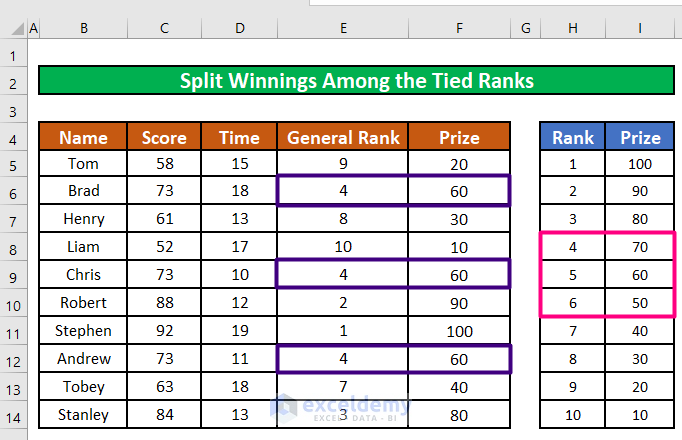
- The fourth argument is a COUNTIF function that will find out how many times the value in E5 appears in the expanding range $E$5:$E$14. The value returned by the COUNTIF function will tell the OFFSET function how many rows it should refer to (the height of the reference). In the case of the 3 cells with tied ranks (cells F6, F9, F12), it will return 3. The COUNTIF function will find the rank 4 in the expanding range 3 times. So, in the case of these 3 cells, the OFFSET function will refer to 3 cells: I8, I9, and I10, as the height of the reference is 3. These 3 cells respectively refer to the prize assigned to the ranks 4, 5, and 6.
- Finally, the AVERAGE function will average the cell values that the OFFSET function returns. In the case of the 3 cells with tied ranks, it will average the values in I8, I9, and I10. Each participant holding the tied ranks will receive this average prize money.
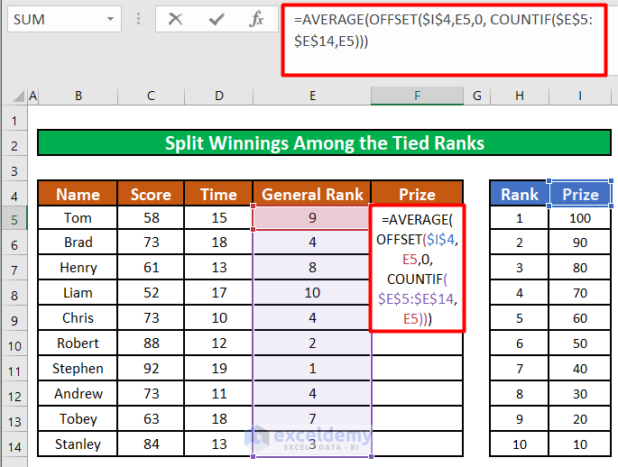
Tom, who ranked 9th in this list, has $20 (the correct prize specified for the 9th position).
- Drag the fill handle of cell F5 to apply the formula to the rest of the cells.
Each of the 3 participants holding the 4th position has received the average of the 3 prizes specified for the 4th, 5th, and 6th (70+60+50 = 180. 180/3 = 60).
Method 5 – Using the SUMPRODUCT Function To Prevent Skipping Ranks in Excel
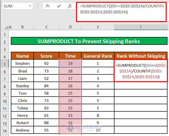
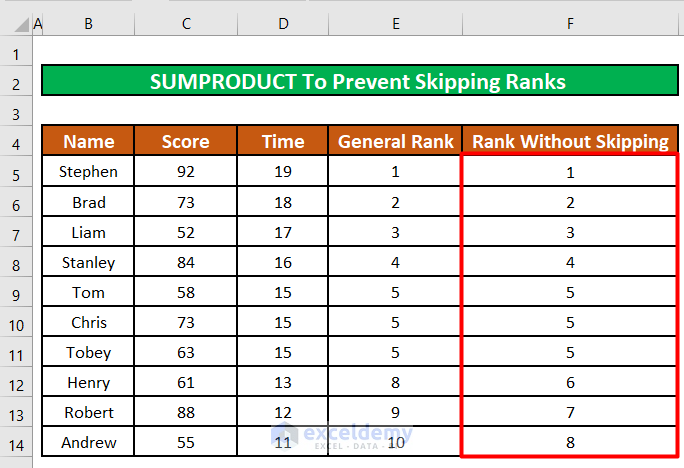
Suppose we do not want to break the tie in a rank, but we also want to prevent the RANK function from skipping the succeeding ranks. For example, we have a 3-way tie in 5th place, so the RANK formula will skip the 6th and 7th positions, because the 2 participants supposed to hold these ranks are now in 5th. We want to still have 6th and 7th positions but without breaking the tie in the 5th position.
Steps:
- Enter the below formula in cell F5:
=SUMPRODUCT((D5<=$D$5:$D$14)/COUNTIF($D$5:$D$14,$D$5:$D$14))The SUMPRODUCT function will multiply and then sum up the values in the $D$5:$D$14 which are greater than or equal to cell D5 with the values returned by the COUNTIF function.
- Press ENTER.
The rank of the first participant in the list remains unchanged.
- Drag the fill handle of cell F5 to apply the formula to the rest of the cells.
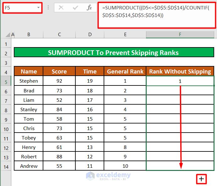
The tie in 5th rank has not been broken. But Excel has not skipped the 6th and 7th positions in the rankings. We now have a total of 8 positions or ranks instead of the original 10 ranks for 10 participants.
Things to Remember
- The article has links to the tutorials on each of the functions we have used. Please visit the pages to learn about these functions.
Download Practice Workbook
Related Articles
- Excel Formula to Rank with Duplicates
- How to Rank in Excel Highest to Lowest
- How to Calculate Top 10 Percent in Excel
- How to Rank Within Group in Excel
- Ranking Data in Excel with Sorting
<< Go Back to Excel RANK Function | Excel Functions | Learn Excel
Get FREE Advanced Excel Exercises with Solutions!


Thank you for your EXCELlent website!
Wish you can help me with my problem, because I am at a loss…
I’m trying to create a scorecard for 20 players who play 22 games.
I need 24 tie breakers:
– 22 Tie breakers for the positions in which they have finished the game;
– 1 Tie breaker for the number of games they have played;
– 1 Arbitrary tie breaker in case everything is tied.
In case the points are tied, then the best position must be checked.
If also the best positions are tied, then the second best must be checked, etc. (up to 22 games).
Let’s say that after 3 games two players are both equal in points and in positions, then the “Arbitrary tie breaker” comes into play.
In case that after 3 games two players are equal in points and positions, but one player has only played 2 games and the other one has played 3 games, the player who played 3 games must be ranked higher.
The names of the players are in columns E40:E60.
Their points are in GU40:GU60.
In GV40:GV60 I have the best positions per player.
In GW40:GW60 the second best positions, … in HQ40:HQ60 the 22nd best position.
In HR40:HR60 I have the number of games played per player.
In HS40:HS60 the total of games played.
In HT40:HT60 the percentage of games played per player.
I wish that it is clear what I want and that you can help me.
Thank you very much in advance!
Gr. Anthoney.
Hi ANTHONEY,
Thanks for your comment. You requirement needs the Excel file. Please share your Excel file and repost your problem on our official ExcelDemy Forum. Our experts will try to reach you out.
Regards
Rafiul Hasan
Team ExcelDemy
Hello
I am trying to rank students scores in 3 groups, for example (A2:A21,A22:A43,A44:62).I don’t use table and I also would like the Range works dynamic, that’s when the ranges exchange from A2:A21 to A2:A25 and A22:A43 to A26:A50 and so on, the formula works correctly.
If two students have the same score they will receive the same rank. For example 20=1,20=1 , 19.25=2 and 19=3
Hello JOHN,
Thanks for your comment. If new value is inserted in the range, the range changes (for example, from A2:A21 to A2:A25). You want to make the formula dynamic for the changed range. It seems you don’t want to use table. Actually, without using table, you won’t be able to make the formula dynamic.
The RANK function and the RANK.EQ function allow you to make the rank dynamic. But these functions assign the same rank to tied numbers and does not leave gaps in the ranking sequence. For example, if there is a tie for the second and third positions, both positions will be assigned a rank of 2, and the next distinct number will be ranked 4. But if you want to fill the next rank after ties, these functions are not useful. In that case, you have to use any of the methods stated in the article and copy the formula for the newly inserted value in the range. Without using table, it is not possible to make the formula dynamic.
Regards
Rafiul Hasan
Team ExcelDemy