In this article, we’ll use a dataset of sales from some sales representatives to demonstrate how to rank in Excel highest to lowest in 13 different cases.
Download Practice Workbook
You can download the Excel workbook that we used to prepare this article.
How to Rank in Excel Highest to Lowest (13 Handy Examples)
Method 1 – Rank from Highest to Lowest with Singular Criteria in Excel
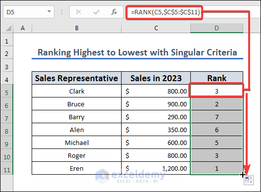
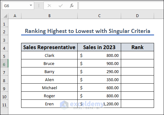
Let’s rank the salespeople based on the total sales in column C, sorting from highest to lowest.
- Apply the following formula to D5 and drag the fill handle from D5 to D11.
=RANK(C5,$C$5:$C$11)
The RANK function will rank the value in cell C5 according to its position in the range C5:C11, from the highest value down. The function will return the rank of the value in cell C5 as a number. For instance, the function will return 2 if cell C5 contains the second-largest value in the range.
When we write the formula with the $ symbol for a cell, we put an absolute reference to the range C5:C11 so it doesn’t change with AutoFill.

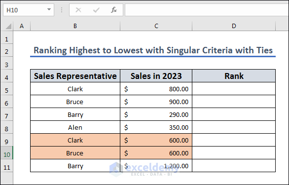
Method 2 – Rank from Highest to Lowest with Singular Criteria with Ties
Let’s use a similar approach to account for ties in the dataset, such as the rows 9 and 10 in the following dataset.
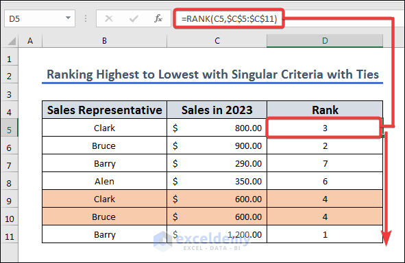
- Apply the following formula in D5 and drag and drop the fill handle to D11:
=RANK(C5,$C$5:$C$11)
In this case, we have ties in Bruce(B9) and Clark(B10), so they are ranked the same.
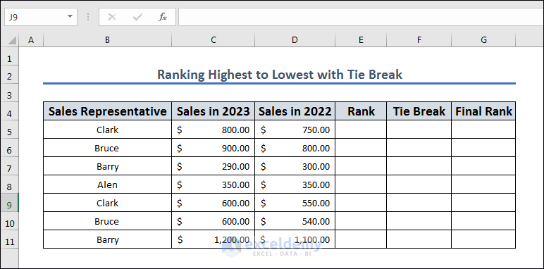
Method 3 – Rank from Highest to Lowest with Tie Break
Let’s expand the previous dataset with past year’s sales to use for breaking any ties in ranking.
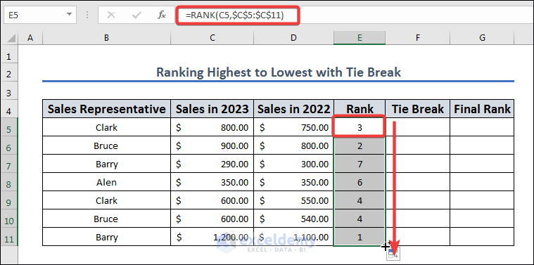
- Create regular ranking based on “Sales in 2023.” In the E5 cell, apply the following formula and fill from E5 to E11 by dragging and dropping the fill icon:
=RANK(C5,$C$5:$C$11)
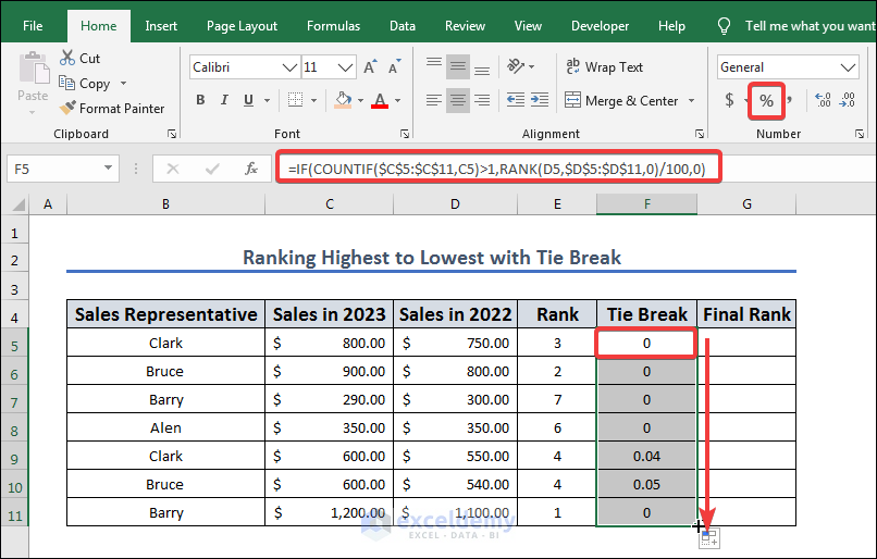
- To create tie breaks, apply the following formula in cell F5 and drag the fill icon F5 to F11.
=IF(COUNTIF($C$5:$C$11,C5)>1,RANK(D5,$D$5:$D$11,0)/100,0)
Formula Breakdown
The formula =IF(COUNTIF($C$5:$C$11,C5)>1,RANK(D5,$D$5:$D$11,0)/100,0) checks if there are any duplicates of the value in cell C5 within the range $C$5:$C$11. If there are duplicates, it calculates the rank of the value in cell D5, relative to the range of values $D$5:$D$11, and divides the result by 100. If there are no duplicates, the formula returns 0. More specifically, the COUNTIF function counts the number of times the value in cell C5 appears in the range $C$5:$C$11. If this count is greater than 1 (indicating that there are duplicates), the RANK function calculates the rank of the value in cell D5, relative to the range $D$5:$D$11, in descending order (the 0 as the third argument specifies this). The resulting rank is then divided by 100. If the count is not greater than 1, the formula returns 0.
- Add the Tie Break and Rank in the G5 cell to get the final rank by applying the following formula in the cell:
=E5+F5
- AutoFill column G based on cell G5.
![]()
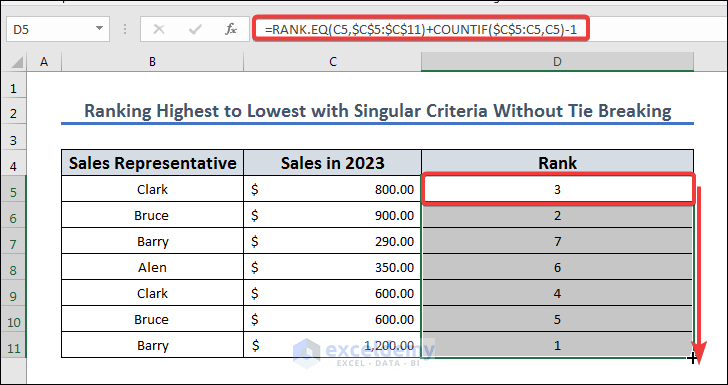
Method 4 – Rank from Highest to Lowest with Singular Criteria Without Tie Breaking
We are going to use the dataset given below to rank the dataset without any tie breaking.
![]()
- Copy the following formula to cell D5, apply it, and then drag and drop the fill icon from D5 to D11:
=RANK.EQ(C5,$C$5:$C$11)+COUNTIF($C$5:C5,C5)-1
Formula Breakdown
The RANK.EQ function calculates the rank of the value in cell C5 relative to the range $C$5:$C$11, where equal values receive the same rank and the next rank is skipped. The COUNTIF function counts the number of times the value in cell C5 appears within the range $C$5:C5 (up to the current row), and subtracts 1 from that count. This adjustment ensures that if there are duplicates of the value in cell C5 above it in the range, the rank is adjusted accordingly.
By adding the result of the RANK.EQ function to the result of the COUNTIF function (minus 1), the formula calculates the final rank of the value in cell C5, accounting for any ties or duplicates in the range.
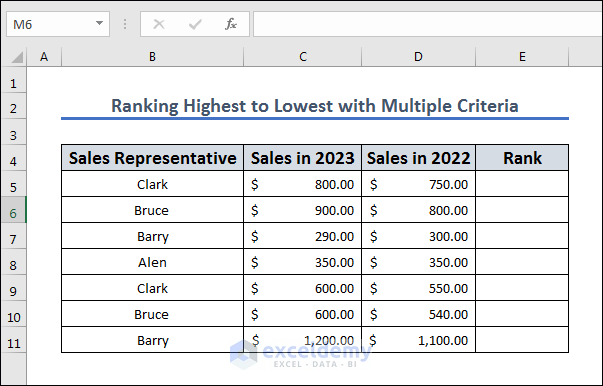
Method 5 – Rank from Highest to Lowest with Multiple Criteria
Let’s use two years’ worth of sales to determine the rankings.
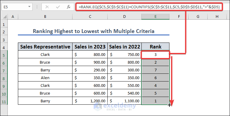
- Copy this formula in the E5 cell:
=RANK.EQ($C5,$C$5:$C$11)+COUNTIFS($C$5:$C$11,$C5,$D$5:$D$11,">"&$D5)
- Press Enter and drag and drop the fill icon from E5 to E11.
Formula Breakdown
The formula calculates the rank of the value in cell C5, taking into account ties or duplicates within the range $C$5:$C$11 and considering the corresponding values in column D.
The RANK.EQ function calculates the rank of the value in cell C5 relative to the range $C$5:$C$11, where equal values receive the same rank and the next rank is skipped. The COUNTIFS function counts the number of times the value in cell C5 appears within the range $C$5:$C$11 and also checks the corresponding values in column D to see if they are greater than the value in cell D5. This adjustment ensures that if there are duplicates of the value in cell C5, the rank is adjusted accordingly based on their corresponding values in column D.
By adding the result of the RANK.EQ function to the result of the COUNTIFS function, the formula calculates the final rank of the value in cell C5.
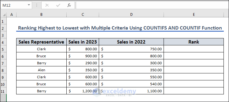
Method 6 – Rank from Highest to Lowest with Multiple Criteria Using COUNTIFS and COUNTIF Functions
Let’s take a dataset where we need to rank with multiple criteria like in Method 3, but instead of tie-breaking individually, we are going to rank them in one go.
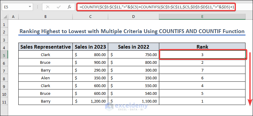
- Insert the following formula in the result cell E5:
=COUNTIF($C$5:$C$11,">"&$C5)+COUNTIFS($C$5:$C$11,$C5,$D$5:$D$11,">"&$D5)+1
- Press Enter and AutoFill to the rest of the column.
Formula Breakdown
The formula counts the number of cells in the range $C$5:$C$11 that have a higher value than cell C5 and the number of cells in the same range that have the same value as C5 and also have a value greater than cell D5, and then adds 1 to the total count.
More specifically, the COUNTIF function counts the number of cells in the range $C$5:$C$11 that is greater than the value in cell C5. The “>&” operator means “greater than”, so this function counts the number of cells in the range that have a value greater than the value in cell C5.
The COUNTIFS function counts the number of cells in the range $C$5:$C$11 that have the same value as C5 and also have a value greater than the value in cell D5. The “&” operator is used to concatenate the “>” operator and the value in cell D5, so the function counts the number of cells in the range that have a value greater than the value in cell D5 and also have the same value as C5.
By adding the results of the COUNTIF and COUNTIFS functions and adding 1 to the total count, the formula calculates the final count of cells in the range $C$5:$C$11 that is greater than the value in cell C5, taking into account cells that have the same value as C5 and also have a value greater than the value in cell D5.
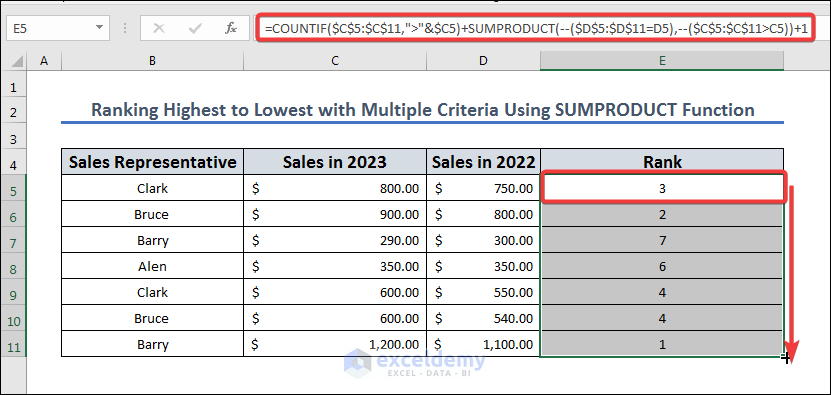
Method 7 – Rank from Highest to Lowest with Multiple Criteria Using the SUMPRODUCT Function
Let’s use a different formula for a similar dataset.
![]()
- Insert the following formula in E5:
=COUNTIF($C$5:$C$11,">"&$C5)+SUMPRODUCT(--($D$5:$D$11=D5),--($C$5:$C$11>C5))+1
- Press Enter and AutoFill to the entire column.
Formula Breakdown
The formula counts the number of cells in the range $C$5:$C$11 that is greater than the value in cell C5, and also counts the number of cells in the same range that have the same value as D5 and also have a value greater than the value in cell C5, and then adds 1 to the total count.
More specifically, the COUNTIF function counts the number of cells in the range $C$5:$C$11 that is greater than the value in cell C5. The “>&” operator means “greater than”, so this function counts the number of cells in the range that have a value greater than the value in cell C5.
The SUMPRODUCT function is used to count the number of cells in the range $C$5:$C$11 that have the same value as D5 and also have a value greater than the value in cell C5. The “–” operator is used to convert the logical TRUE/FALSE values to 1/0 values, and then the two arrays are multiplied together and summed. This results in a count of the number of cells in the range that meet both criteria.
The formula then adds 1 since the counts will give a ranking one below the required. For example, the top result fulfills none of the first two criteria, so its rank becomes 1.
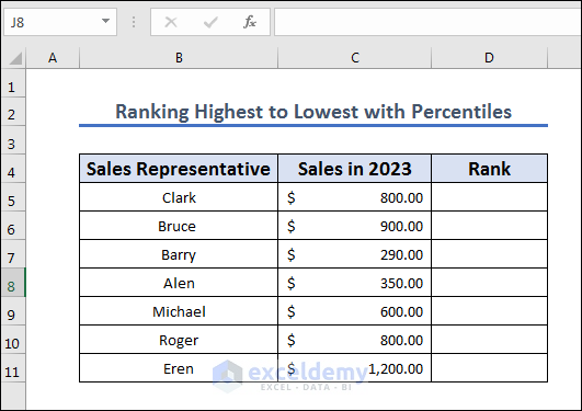
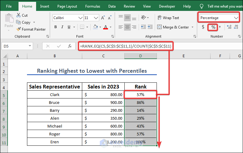
Method 8 – Rank from Highest to Lowest with Percentiles
Let’s use the dataset for a single year’s sales and rank the salespeople as a percentile of the sample.
- Copy the following formula into the result cell D5.
=RANK.EQ(C5,$C$5:$C$11,1)/COUNT($C$5:$C$11)
- Press Enter and use the Fill Handle tool to AutoFill to the other cells in the column.
Formula Breakdown
The formula calculates the relative rank of the value in cell C5 within the range $C$5:$C$11. The “1” argument in the RANK.EQ function specifies that ties are ranked as the average of the ranks of the tied values. The result of the RANK.EQ function is divided by the total count of values in the range $C$5:$C$11 to normalize the rank.
The formula is used to compare the value in cell C5 to the other values in the range $C$5:$C$11 and determine its relative position. The result will be a number between 0 and 1, where a value of 0 means that the value in cell C5 is the smallest value in the range, and a value of 1 means that the value in cell C5 is the largest value in the range. The relative rank of a value can be useful in analyzing data and making comparisons between different values.
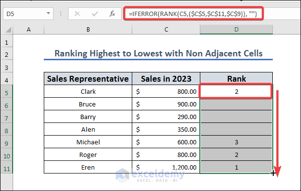
Method 9 – Rank from Highest to Lowest with Non-Adjacent Cells
In this section, we are going from highest to lowest with a non-adjacent dataset. We will use the same dataset but use a limited selection.
![]()
- Copy the following formula to D5:
=IFERROR(RANK(C5,($C$5,$C$11,$C$9)), "")
- Press Enter and use the Fill Handle to AutoFill to the rest of the column.
Formula Breakdown
The formula returns the rank of the value in cell C5 within the range $C$5,$C$11,$C$9. If the rank can’t be calculated, the formula returns an empty string (“”).
The RANK function calculates the rank of the value in cell C5 within the specified range, where the highest value has a rank of 1, the second highest has a rank of 2, and so on. The range is specified as an array containing the values $C$5, $C$11, and $C$9. If the value in cell C5 is not found in the specified range, the RANK function will return an error.
The IFERROR function is used to handle the error that may occur if the value in cell C5 is not found in the specified range. If an error occurs, the IFERROR function returns an empty string (“”) instead of the error message. This can be useful to avoid displaying an error message to the user and to make the output more visually appealing.
Method 10 – Rank from Highest to Lowest According to a Group in Excel
Let’s put the salespeople in two groups (A and B, listed in column B) and rank them within their group.
![]()
- Copy the following formula to cell E5.
=SUMPRODUCT((B5=$B$5:$B$11)*(D5<$D$5:$D$11))+1
- Press Enter and use AutoFill on other cells in the column.

Formula Breakdown
=SUMPRODUCT((B5=$B$5:$B$11)*(D5<$D$5:$D$11))+1
- SUMPRODUCT(): This is a function that multiplies corresponding values in arrays and returns the sum of those products.
- (B5=$B$5:$B$11): This is an array that returns TRUE or FALSE for each cell in the range B5:B11, depending on whether the value in that cell is equal to the value in B5.
- (D5<$D$5:$D$11): This is another array that returns TRUE or FALSE for each cell in the range D5:D11, depending on whether the value in that cell is less than the value in D5.
- *(asterisk): This operator is used to multiply the two arrays element-wise, which means it multiplies the corresponding elements in both arrays and returns an array of the same size as the original arrays.
- +1: This adds 1 to the sum of the products of the two arrays.
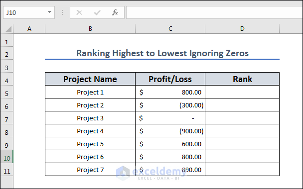
Method 11 – Rank From Highest to Lowest Ignoring Zeroes
The Rank function can provide errors if the dataset has no value. Let’s insert a zero value in the dataset and use a modified formula to avoid ranking it.
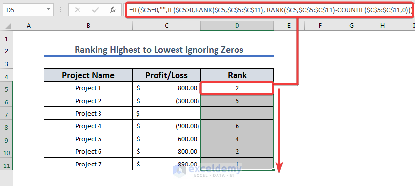
- Copy the following formula into D5.
=IF($C5=0,"",IF($C5>0,RANK($C5,$C$5:$C$11),RANK($C5,$C$5:$C$11)-COUNTIF($C$5:$C$11,0)))
- Press Enter and drag the fill icon from D5 to D11.
Formula Breakdown
IF($C5=0,””,IF($C5>0,RANK($C5,$C$5:$C$11),RANK($C5,$C$5:$C$11)-COUNTIF($C$5:$C$11,0)))
- IF($C5=0,””,…): This is an outer IF statement that checks if the value in cell C5 is equal to zero. If it is, it returns an empty string (“”). If it isn’t, it proceeds to the inner IF statement.
- IF($C5>0,…): This is an inner IF statement that checks if the value in cell C5 is greater than zero. If it is, it returns the rank of the value in the range C5:C11. If it isn’t, it proceeds to the else part of the IF statement.
- RANK($C5,$C$5:$C$11): This function returns the rank of the value in cell C5, compared to the values in the range C5:C11.
- RANK($C5,$C$5:$C$11)-COUNTIF($C$5:$C$11,0): This function returns the rank of the value in cell C5, compared to the values in the range C5:C11, and subtracts the count of cells in that range that contain zero.
If the sales figure in cell C5 is zero, the formula returns an empty string (“”). If it’s greater than zero, the formula returns the rank of that value in the range C5:C11. Lastly, if it’s less than or equal to zero, the formula returns the rank of that value in the range C5:C11 but subtracts the count of cells in that range that contain zero. This ensures that zero values are ranked lower than non-zero values.
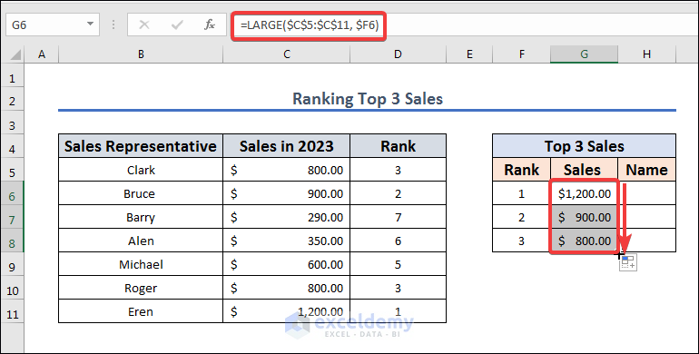
Method 12 – Rank Top 3 Sales from Highest to Lowest in Excel
Let’s extract the three best performers from the dataset.
![]()
- Sort the table with one of the previous methods.
- Insert the following in cell G6.
=LARGE($C$5:$C$11, $F6)
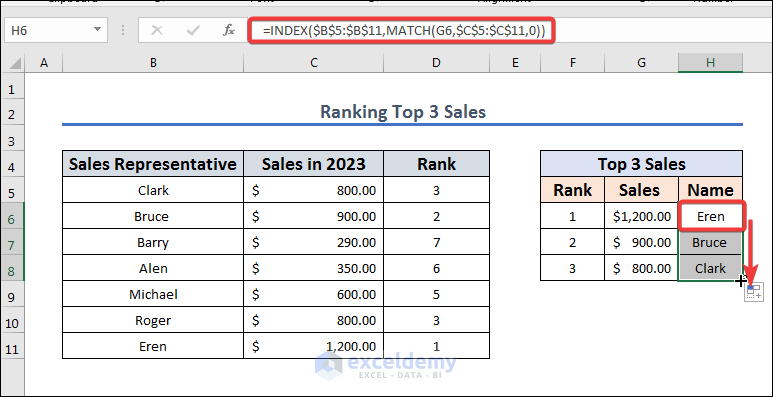
- Input the following formula in H6.
=INDEX($B$5:$B$11,MATCH(G6,$C$5:$C$11,0))
- Apply both formulas and use AutoFill to fill the other rows.
Formula Breakdown
= INDEX($B$5:$B$11, MATCH(G6, $C$5:$C$11, 0))
INDEX(): This is a function that returns a value from a specified row and column in a range.
$B$5:$B$11: This is the range of cells that contains the values we want to return.
MATCH(): This is a function that returns the position of a value in a range.
G6: This is the value we want to find the position of in the range $C$5:$C$11.
$C$5:$C$11: This is the range of cells that contains the values we want to find the position of the value in G6.
Method 13 – Rank Bottom 3 Sales in Excel from Lowest to Highest
Let’s get the worst performers from the sales team.
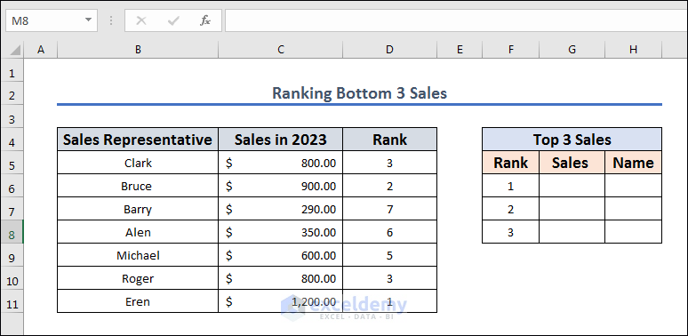
- Rank the table from highest to lowest using one of the methods above.
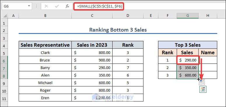
- Insert the following formula in cell G6 and apply it with Enter.
=SMALL($C$5:$C$11, $F6)
Formula Breakdown
The formula SMALL($C$5:$C$11, $F6) is an Excel formula that returns the kth smallest value from a range of cells. Here’s what each part of the formula means:
- SMALL() returns the k-th smallest value from a range of cells.
- $C$5:$C$11 is the range of cells from which the k-th smallest value will be returned. In this case, the range is fixed as an absolute reference using the dollar signs, meaning that the range will not change when the formula is copied to other cells.
- $F6 is the k value that specifies which smallest value should be returned from the range. In this case, the k value is also fixed as an absolute reference, so it will not change when the formula is copied to other cells.
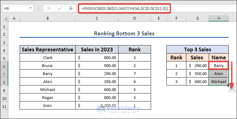
- Copy the following formula in H6 to extract the name based on the sales value.
=INDEX($B$5:$B$11,MATCH(G6,$C$5:$C$11,0))
- AutoFill both formulas down.
Formula Explanation
This formula finds a value in one range and returns the value from the other range that corresponds to that value. What each component of the formula signifies is as follows:
- INDEX() returns a value or reference to a value from within a table or range.
- $B$5:$B$11 is the range of cells from which the function will return a value. In this case, the range is fixed as an absolute reference using the dollar signs, meaning that the range will not change when you copy the formula to other cells.
- MATCH() searches for a specified item in a range of cells, and returns the relative position of the item within the range.
- G6 is the value that the MATCH() function is searching for within the range $C$5:$C$11. In this case, the value is in cell G6.
- $C$5:$C$11 is the range of cells in which the MATCH() function will search for the value G6. In this case, the range is fixed as an absolute reference using the dollar signs, meaning that the range will not change when the formula is copied to other cells.
- 0 is an optional argument that specifies the type of match we want to use. A value of 0 indicates an exact match.
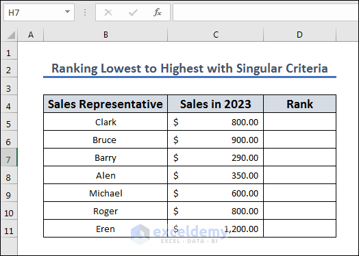
How to Rank Lowest to Highest with Singular Criteria in Excel
Let’s rank the team from lowest to highest.
- Use the following formula in D5 to get the lowest to the highest ranking.
=RANK(C5,$C$5:$C$11,1)
- AutoFill to the other cells in the column.

Formula Breakdown
We use the RANK() function in Excel to determine the rank of a value within a range of values. The formula =RANK(C5,$C$5:$C$11,1) specifically calculates the rank of the value in cell C5 within the range of cells $C$5:$C$11, where the smallest value in the range is assigned a rank of 1.
Here’s a breakdown of the formula:
- C5 is the cell reference to the value for which we want to calculate the rank. In this case, it’s assumed that the formula is located in a different cell than C5.
- $C$5:$C$11 is the range of cells in which we want to calculate the rank of the value in cell C5. The $ signs before the row and column references make this an absolute reference, meaning that it will not change when you copy the formula to other cells.
- 1 is an optional argument that indicates the order in which the function will calculate the rank. A value of 1 means that it will rank the smallest value in the range as 1, the second-smallest as 2, and so on.
Frequently Asked Questions
How do I rank data in Excel?
To rank data in Excel, you can use the RANK function. This function assigns a rank to each value in a list based on its position relative to the other values in the list. The rank of a value is determined by comparing it to the other values in the list.
How do I use the RANK function in Excel?
To use the RANK function in Excel, you need to provide two arguments: the first argument is the value you want to rank, and the second argument is the range of cells containing the values you want to rank against. The function will return the rank of the value within the range.
How do I rank data in Excel with ties?
When there are ties in the data, meaning multiple values have the same value, the RANK function will assign the same rank to each of the tied values, and then skip the next rank.
For example, if two values tie for second place, it will rank them both as assigned a rank of 2, and the next value as a rank of 4.
If you want to assign different ranks to tied values, you can use the RANK.EQ or RANK.AVG functions instead. The RANK.EQ function assigns the same rank to tied values and the RANK.AVG function assigns an average rank to tied values.
Things to Remember
- When using the RANK function, you need to provide at least two arguments: the first argument is the value you want to rank, and the second argument is the range of cells containing the values you want to rank against.
- To rank data from highest to lowest, you can use the RANK function in combination with the COUNT function. The formula is “=COUNT($A$1:$A$10)-RANK(A1,$A$1:$A$10)+1”. This formula will return the rank of the value in A1 within the range A1:A10, with the highest value being ranked as 1.
- When there are ties in the data, the RANK function will assign the same rank to each of the tied values, and then skip the next rank. If you want to assign different ranks to tied values, you can use the RANK.EQ or RANK.AVG functions instead.
- When using the COUNT function in combination with the RANK function, it’s important to use absolute references (e.g. $A$1:$A$10) to ensure that the range doesn’t change when you copy the formula to other cells.
- To make the ranked data easier to read, you can use custom formatting to apply different colors or styles to the top-ranked values. You can do this by selecting the cells containing the ranked data, and then clicking on “Conditional Formatting” in the “Home” tab of the Excel ribbon.
<< Go Back to Excel RANK Function | Excel Functions | Learn Excel
Get FREE Advanced Excel Exercises with Solutions!
