Method 1 – Create an Auto Ranking Table for Ascending Order
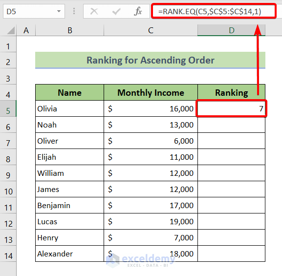
❶ Insert the following formula in cell D5.
=RANK.EQ(C5,$C$5:$C$14,1)❷ Press ENTER.
❸ Drag the Fill Handle icon from cell D5 to D14.
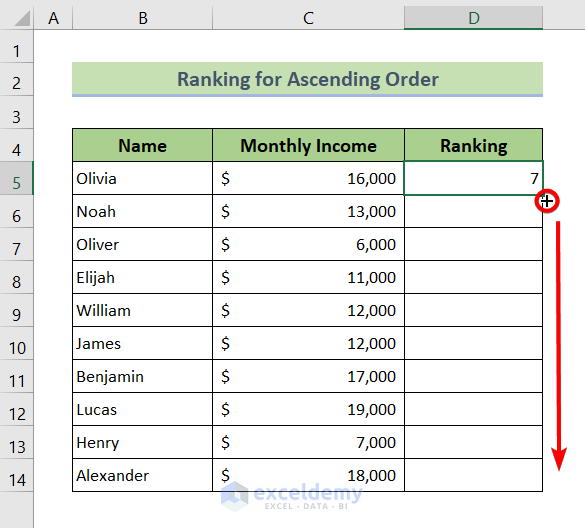
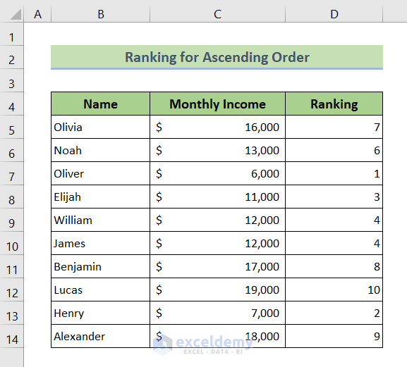
You will see the relative ranking of the data from the Monthly Income column to the Ranking column.
Formula Breakdown
➤ C5
This is the top cell of the range $C$5:$C$14.
➤ $C$5:$C$14
This is the range within which the ranking is performed.
➤ 1
This value refers to the ascending order.
➤ RANK.EQ(C5,$C$5:$C$14,1)
The RANK.EQ function returns the relative ranking of C5 within the range $C$5:$C$14 based on ascending order.
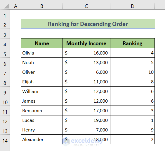
Method 2 – Create an Auto Ranking Table for Descending Order
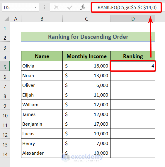
❶ Insert the following formula in cell D5.
=RANK.EQ(C5,$C$5:$C$14,0)❷ Press ENTER.
❸ Drag the Fill Handle icon from cell D5 to D14.
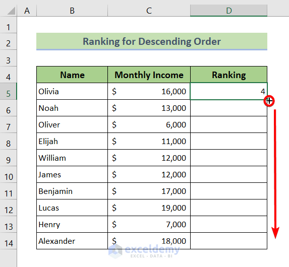
You will see the relative ranking of the data from the Monthly Income column to the Ranking column.
Formula Breakdown
➤ C5
This is the top cell of the range $C$5:$C$14.
➤ $C$5:$C$14
This is the range within which the ranking is performed.
➤ 0
This value refers to the descending order.
➤ RANK.EQ(C5,$C$5:$C$14,0)
The RANK.EQ function returns the relative ranking of C5 within the range $C$5:$C$14 based on descending order.
Read More: Excel Percentile Rank Inc vs Exc
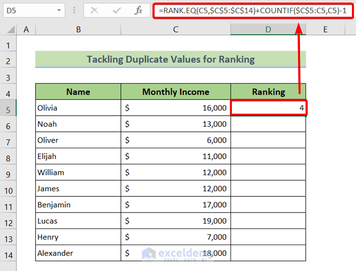
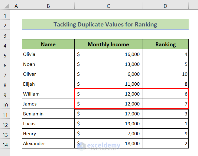
Method 3 – Handle Duplicate Values While Auto Ranking Table in Excel
❶ Insert the following formula in cell D5.
=RANK.EQ(C5,$C$5:$C$14)+COUNTIF($C$5:C5,C5)-1❷ Press ENTER.
❸ Drag the Fill Handle icon from cell D5 to D14.
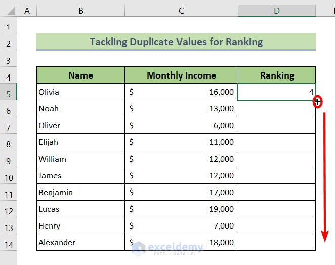
You will see the relative ranking of the data from the Monthly Income column to the Ranking column.
Formula Breakdown
➤ C5
This is the top cell of the range $C$5:$C$14.
➤ $C$5:$C$14
This is the range within which the ranking is performed.
➤ RANK.EQ(C5,$C$5:$C$14)
The RANK.EQ function returns the relative ranking of C5 within the range $C$5:$C$14 based on descending order.
➤ COUNTIF($C$5:C5,C5)
C5 of $C$5:C5 changes as you copy down the formula. The COUNTIF function compares C5 within the range $C$5:C5 for duplicate values and returns the count for the duplicate values.
➤ RANK.EQ(C5,$C$5:$C$14)+COUNTIF($C$5:C5,C5)-1
For any duplicate values, COUNTIF($C$5:C5,C5) returns the occurrence of the duplicates which is added to the rank returned by RANK.EQ(C5,$C$5:$C$14). 1 is subtracted to keep the original ranking of the data.
Related Articles
- How to Calculate Rank Percentile in Excel
- How to Rank in Excel Highest to Lowest
- How to Stack Rank Employees in Excel
- How to Create a Ranking Graph in Excel
- How to Rank Average in Excel
- How to Calculate Weighted Ranking in Excel
<< Go Back to Excel RANK Function | Excel Functions | Learn Excel
Get FREE Advanced Excel Exercises with Solutions!
