Excel Rank Function
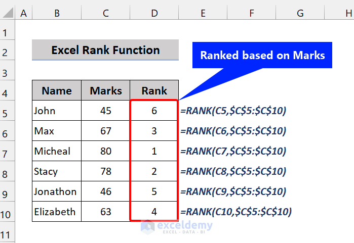
To rank multiple items there is a built-in Excel RANK Function, which ranks multiple values based on a column that you specify, in either ascending or descending order.
What it does is the following:
But it is not possible to rank items based on conditions using this function.
Is it Possible to Rank with Conditions Using a Single Function?
Can we rank numbers, values, and items based on single or multiple criteria simply using the RANK function? Or is there a RANKIF function that exists?
Unfortunately not. There is no RANKIF function in Excel.
However to rank multiple values based on criteria, we can use the COUNTIFS function and the SUMPRODUCT function.
Example 1 – Rank Students’ Marks IF Matches the Group
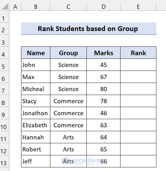
Let’s rank some students’ marks based on their subject group using the COUNTIFS function.
The Generic formula we are going to use is:
=COUNTIFS(criteria_range,criteria,values,”>”&value)+1
Here’s our sample dataset:
Steps:
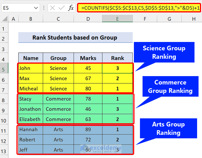
- Enter the following formula in cell E5:
=COUNTIFS($C$5:$C$13,C5,$D$5:$D$13,">"&D5)+1
- Press Enter and drag the Fill handle icon over the range E6:E13.
A rank based on the group is created.
How Does the Formula Work?
The COUNTIFS function executes a conditional count utilizing multiple criteria. We enter those conditions as a criteria range.
=COUNTIFS(C5:C13,C5)
This function returns 3 because there are three science groups.
The second criteria is the following:
=COUNTIFS($C$5:$C$13,C5,$D$5:$D$13,”>”&D5)
This function checks whether the current mark is greater than other marks or not.
=COUNTIFS($C$5:$C$13,C5,$D$5:$D$13,”>”&D5)+1
We add 1 to this equation because when the mark is the highest in that group it will return 0, but we can’t rank starting from zero, so we add 1 to start the ranking from 1.
Remove Duplicates
But there’s a catch. If you have the same marks for two students, it will rank both of them as 1. In so doing, it will create a rank of 3 for the next item. So we will have a ranking of 1,1,3. To remove this confusion, enter the following formula:
=(COUNTIFS($C$5:$C$13,C5)+1-(COUNTIFS($C$5:$C$13,C5,$D$5:$D$13,">"&D5)+1)-(COUNTIFS($C$5:$C$13,C5,$D$5:$D$13,"<"&D5)+1))/2
If there are no duplicates in your dataset, it will return 0.
Read More: How to Rank Within Group in Excel
Example 2 – Reverse the Rank IF Formula
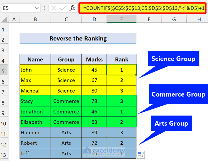
The previous example we showed was in descending order. Let’s reverse this with a simple tweak in the formula: changing the greater than (>) operator to the smaller than (<) operator.
The generic formula:
=COUNTIFS(criteria_range,criteria,values,”<“&value)+1
Steps:
- Enter the following formula in cell E5:
=COUNTIFS($C$5:$C$13,C5,$D$5:$D$13,"<"&D5)+1
- Press Enter and drag the Fill handle icon over the range E6:E13.
A rank based on criteria in descending order is created.
Example 3 – Using Rank-IF Formula for Sales Based on Product
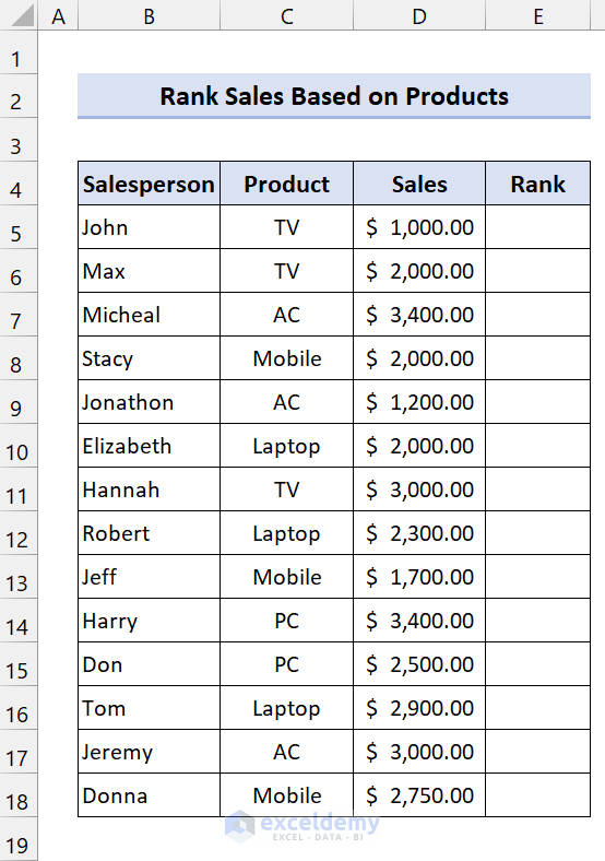
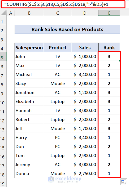
Here’s our dataset, which is slightly different from the previous one:
We have some salesperson’s selling products and their total sales, and will calculate rank based on the products. However, the products are scattered in the dataset. They are not in groups like in the previous example.
Steps:
- Enter the following formula in cell E5:
=COUNTIFS($C$5:$C$18,C5,$D$5:$D$18,">"&D5)+1
- Press Enter and drag the Fill handle icon over the range E6:E13.
A Rank IF formula in Excel is successfully generated.
Example 4 – Rank-IF Formula to Rank Sales Based on Quarters
Let’s apply the previous formula to a table, which allows you to calculate various operations over a dataset.
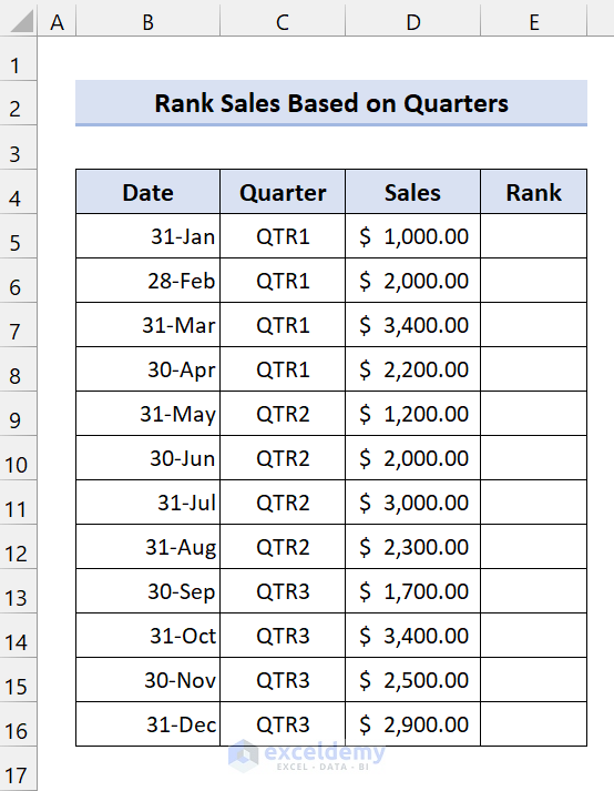
Here’s our dataset:
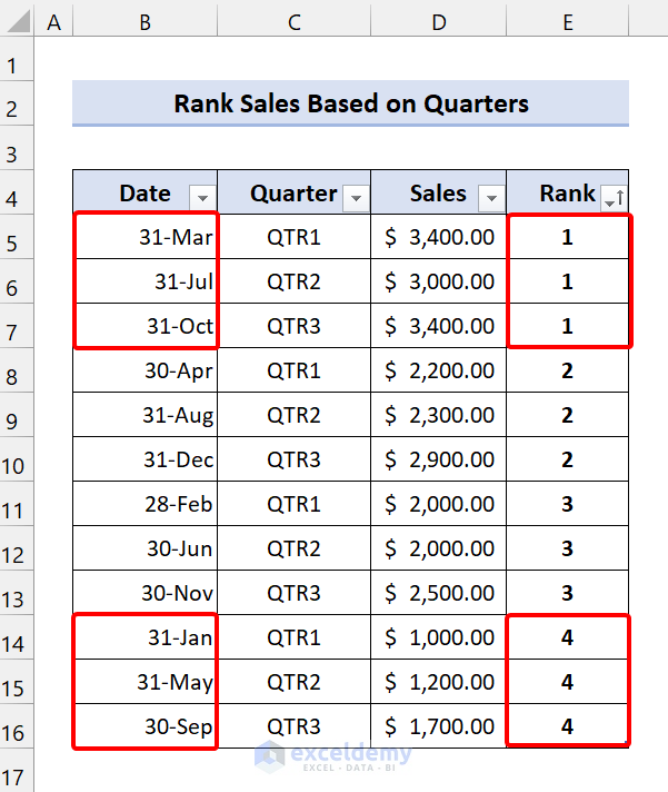
We have some sales data of quarters in a year. Let’s create ranks based on the criteria “Quarter”.
Steps:
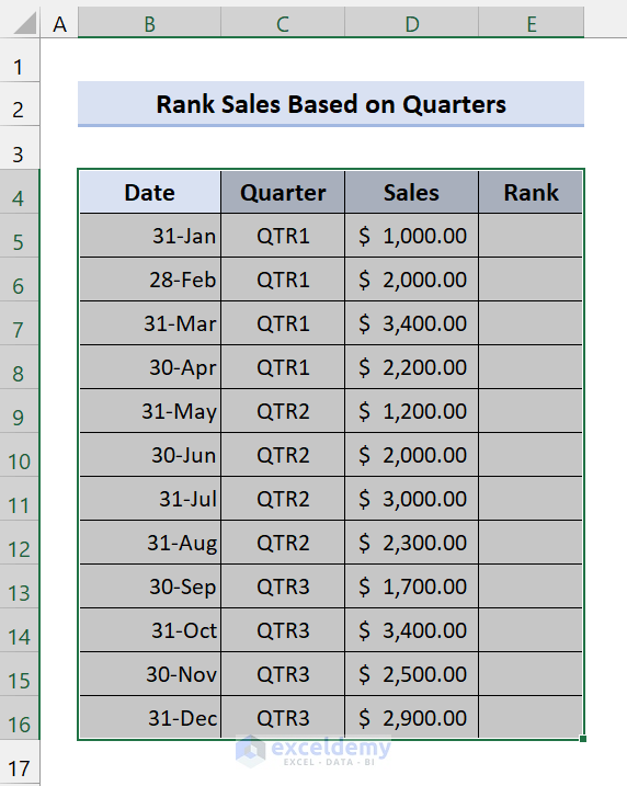
- Select the whole dataset.
- Press Ctrl+T on your keyboard to transform it into a table.
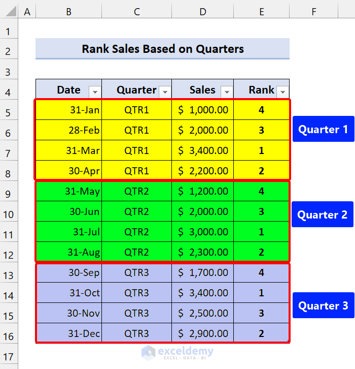
- Type the following formula in cell E5:
=COUNTIFS($C$5:$C$16,C5,$D$5:$D$16,">"&D5)+1
- Press Enter and drag the Fill handle icon over the range E6:E16.
- Perform Sorting or Filtering to see the best-performing month and least-performing month in the quarter.
Read More: Ranking Data in Excel with Sorting
Method 5 – Using SUMPRODUCT Function Instead of RANK-IF
The Generic formula we are going to use:
=SUMPRODUCT((criteria_range=criteria)*(value>values))+1
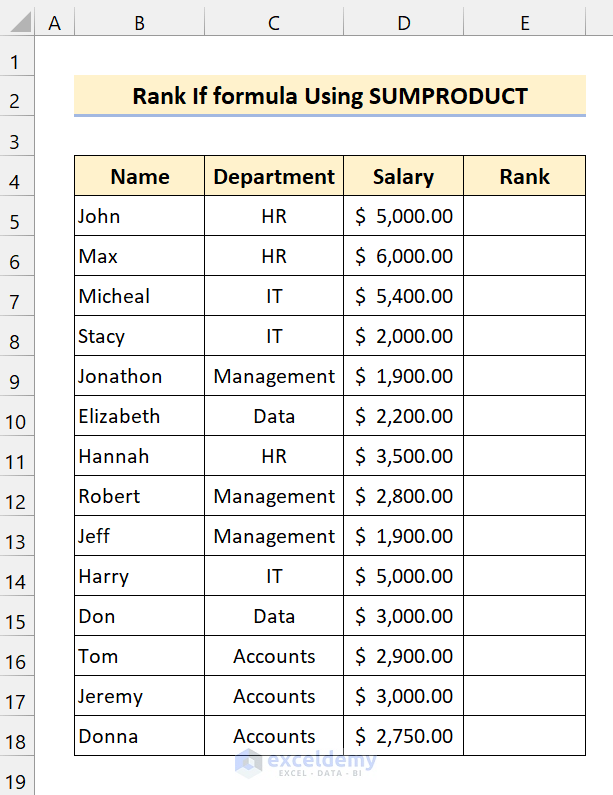
Here’s our dataset:
Let’s calculate the ranks of the Salaries based on Department Salaries. The process is similar to the previous examples, we will just use the SUMPRODUCT function instead of COUNTIFS.
Steps:
- Enter the following formula in cell E5:
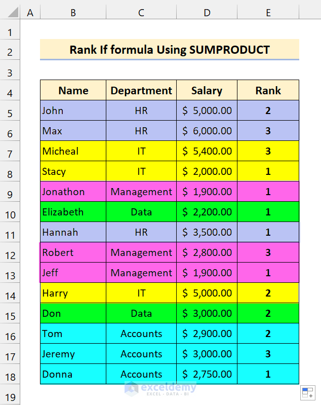
=SUMPRODUCT(($C$5:$C$18=C5)*(D5>$D$5:$D$18))+1
- Press Enter and drag the Fill handle icon over the range E6:E13.
Using color grading, we tried to differentiate the ranking based on the departments.
How Does the Formula Work?
The SUMPRODUCT takes one or more arrays as an argument, multiplies the corresponding values of all the arrays, and then returns the sum of the products. We enter those conditions as a criteria range.
=($C$5:$C$18=C5)
It checks the whole column and finds matches, returning the results in an array. If there are any matches, it returns TRUE, and FALSE for non-matching values.
The second criterion is the following:
=(D5>$D$5:$D$18)
It checks the salary, sorts them in descending order, and returns TRUE for the salaries greater than or equal to D5, and FALSE otherwise. To sort it in ascending order instead, change the greater than symbol (D5<$D$5:$D$18).
=SUMPRODUCT(($C$5:$C$18=C5)*(D5>$D$5:$D$18))+1
The SUMPRODUCT function sums up the values of the 1’s and 0’s array. It returns 0 for the largest number of each group. We added 1 to the outcome to start ranking with 1.
Read More: Excel Formula to Rank with Duplicates
Things to Remember
✎ We demonstrated this article in descending order (largest to smallest). Change the ranking order according to your needs.
✎ Don’t forget to add 1 to the formula, otherwise it will create ranks starting from 0.
✎ Any Rank procedure in Excel works only for numeric values, namely positive and negative numbers, zeros, date, and time values. Non-numeric values will be ignored.
Download Practice Workbook
Related Articles
- Ranking Based on Multiple Criteria in Excel
- How to Rank with Ties in Excel
- How to Rank in Excel Highest to Lowest
- How to Calculate Top 10 Percent in Excel
<< Go Back to Excel RANK Function | Excel Functions | Learn Excel
Get FREE Advanced Excel Exercises with Solutions!