How to Create a Ranking Graph in Excel (5 Methods)

Method 1 – Create a Ranking Graph with Sort Command in Excel

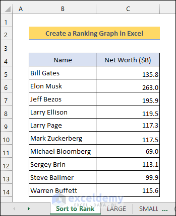
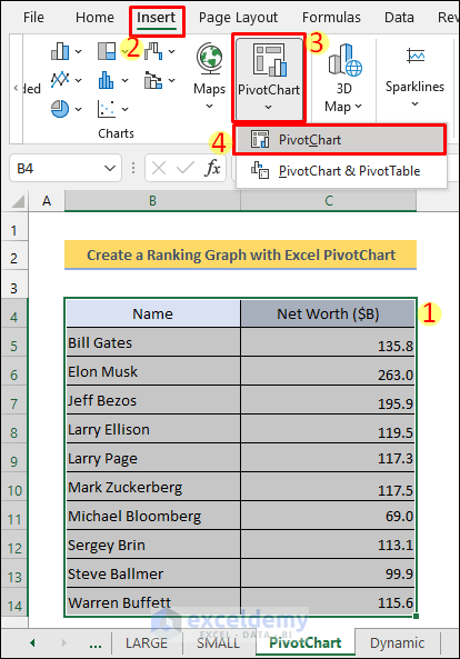
The sample dataset below contains a list of the wealthiest persons in the USA.

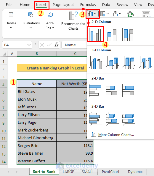
• Select the entire dataset (B4:C14). Select Insert >> 2-D Column as shown in the image below.

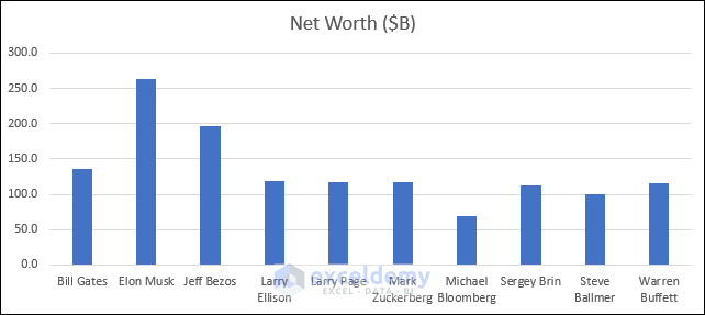
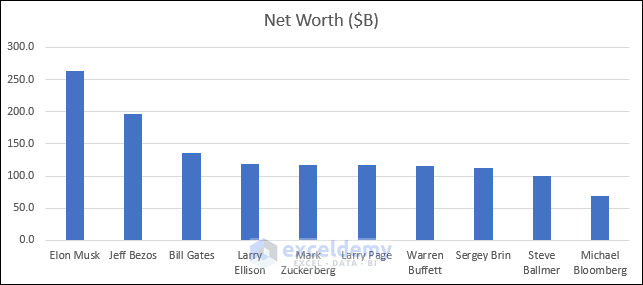
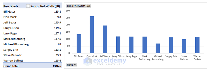
• The graph does not show the data based on the highest to lowest ranking or vice versa.

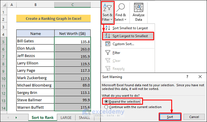
• To solve the problem, select the Net Worth column.
• Select Sort & Filter >> Sort Largest to Smallest from the Home tab as shown below. A warning window will pop up.
• Choose Expand the Selection in the Sort Warning window and hit the Sort button.

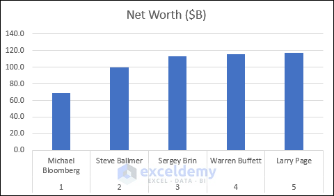
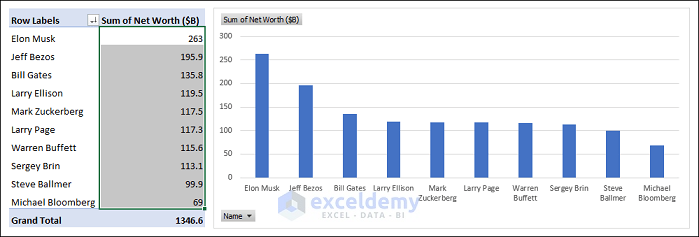
• The graph will look as shown.

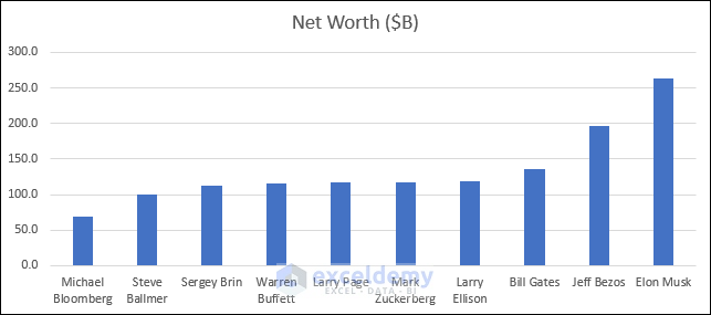
• The data can be sorted from Smallest to Largest.

Read More: How to Stack Rank Employees in Excel

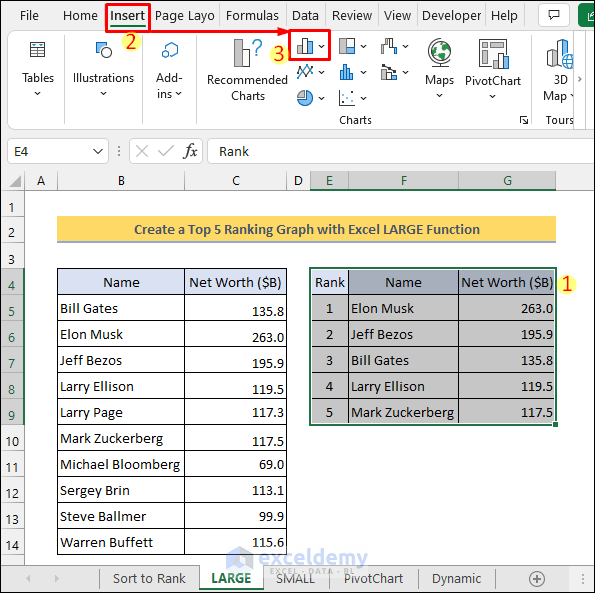
Method 2 – Construct a Ranking Graph with Excel LARGE Function

Steps

• Enter the numbers 1 to 5 in cells E5to E9. Enter the formula below in cell G5. Use the Fill Handle icon to apply the formula to the cells below.

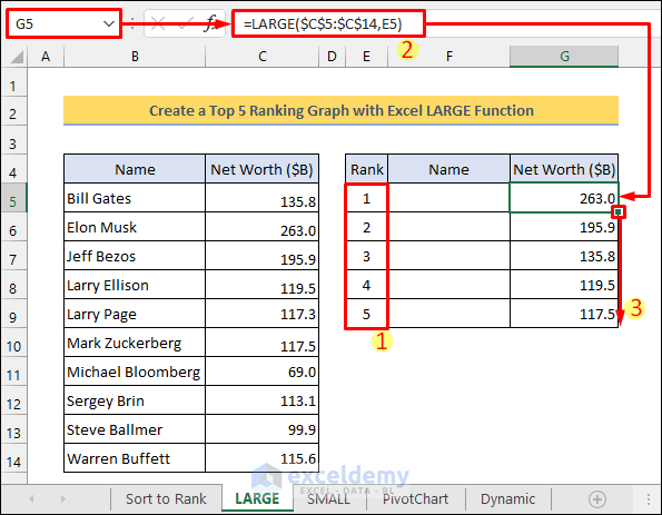
• Input the INDEX-MATCH formula with the functions in cell F5. Drag the Fill Handle icon to the cells below.

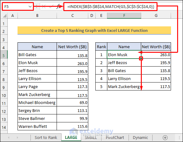
• Select the new dataset (E4:G9) containing the top 5 wealthiest persons. Select Insert >> 2-D Column.

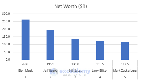
The graph result shows the ranking of the top 5 wealthiest persons as shown in the image below.

Read More: How to Rank Average in Excel

Method 3 – Build a Ranking Graph with Excel SMALL Function

Input the formula below in cell G5.

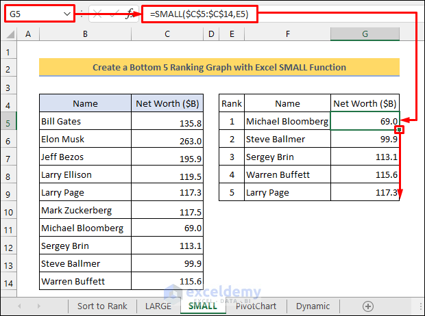
• Insert the chart with the new dataset.

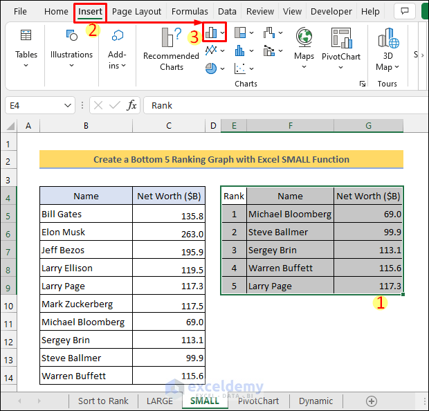
• The ranking graph will look as shown in the image below.

Read More: How to Create an Auto Ranking Table in Excel

Method 4 – Plot a Ranking Graph with Excel PivotChart

Steps

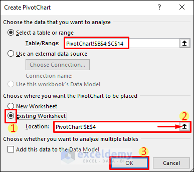
• Select the entire dataset. Select Insert >> PivotChart >> PivotChart as shown below.

• Check the radio button for Existing Worksheet in the Create PivotChart.
• Use the upward arrow in the Location field to select the cell (E4) where you want the PivotChart.
• Click OK.

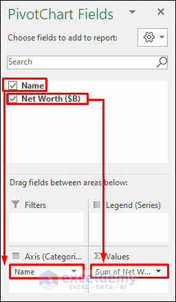
• Drag the Name table in the Axis area and the Net Worth table in the Values area as shown in the image.

• This will create the following PivotChart along with a PivotTable.

• Sort the data in the PivotTable to show the data rank-wise in the graph.

Method 5 – Make a Dynamic Ranking Graph in Excel

Steps:

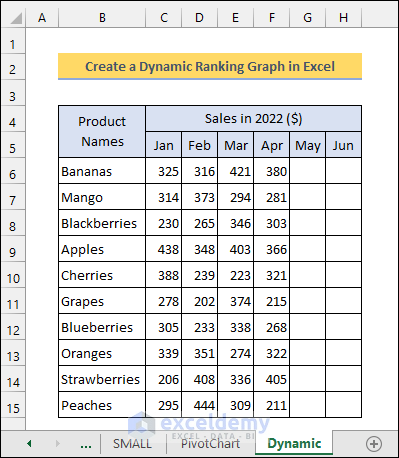
• Assume you have the following dataset. It contains the monthly sales amount of different products. You will need to add more rows and columns to the dataset in the future.

• Enter the following formula in cell I6. Drag the Fill Handle icon to the cells below. The SUM function in the formula will return the total sales for each product.

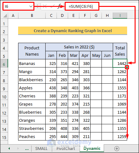
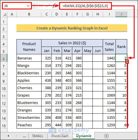
• Apply the following formula in cell J6and to the cells below using the Fill Handle icon.

• The RANK.EQ function returns the ranks of the products based on their total sales amount.

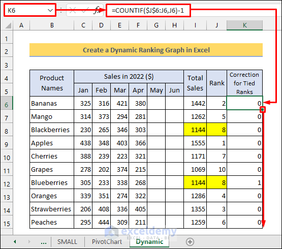
• The function returns the rank 8 twice as the total sales for Blackberries and Blueberries are the same. Enter the following formula in cell K6 to correct this issue.

• The COUNTIF function in the formula checks for repeating values.

• Apply the following formula in cell L6 to get a unique rank for each product.

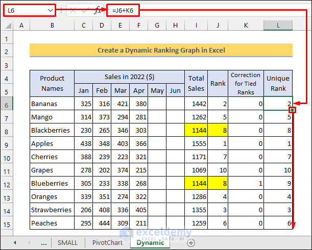
• Enter the numbers 1 to 5 in cells N6 to N10 Then apply the following formula in cell O6 and copy it down.

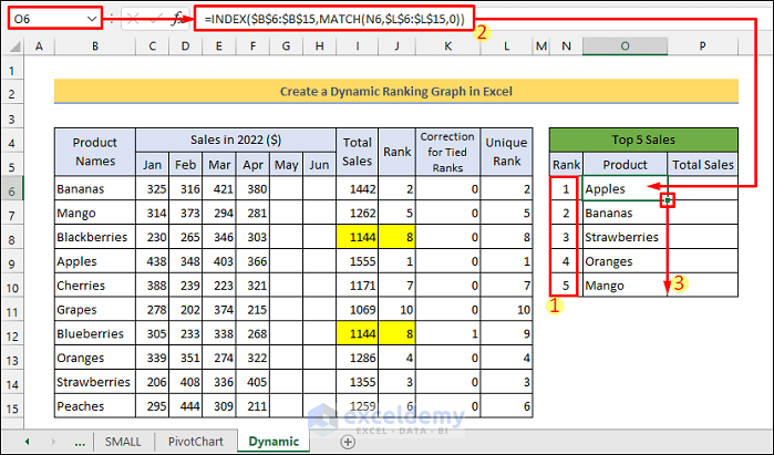
• Enter the following formula in cell P6. Drag the Fill Handle icon to the cells below.

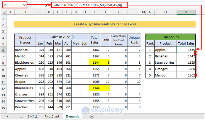
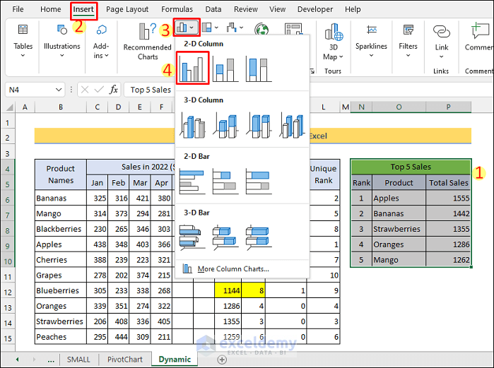
• The dataset for the dynamic ranking graph is ready. Select the dataset (N4:P10). Select Insert >> 2-D Column to create the dynamic graph.

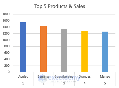
The dynamic ranking graph will appear as shown below.

You can insert new rows between rows 11 and 15 to add more products. You need to use the Fill Handle icon to copy the formulas to the newly added cells. You can also add more columns between columns C and H to add more sales data for the new months in the future. The ranking graph will update automatically.

Download Practice Workbook

Related Articles

• How to Calculate Rank Percentile in Excel
• Excel Percentile Rank Inc vs Exc
• How to Rank in Excel Highest to Lowest
• How to Calculate Weighted Ranking in Excel

<< Go Back to Excel RANK Function | Excel Functions | Learn Excel