How to Rank Data in Excel Using Sorting (3 Methods)

Dataset Overview

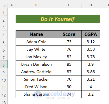
In this guide, we’ll work with a dataset containing student scores in an exam, their current CGPA, and corresponding names.

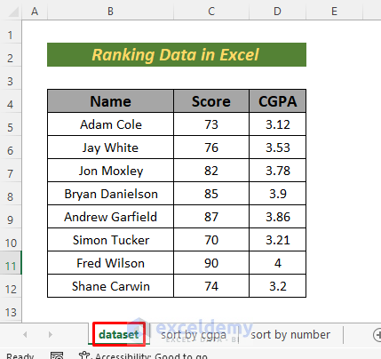
Method 1 – Using SORT and RANK Functions to Rank by Exam Scores

Set Up Your Sheet:
- Create a new sheet with columns for names, scores, and CGPAs.

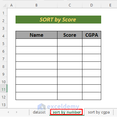
Sorting with SORT Function:
- In cell B5, enter the following formula:

=SORT(dataset!B5:D12,2,-1,FALSE)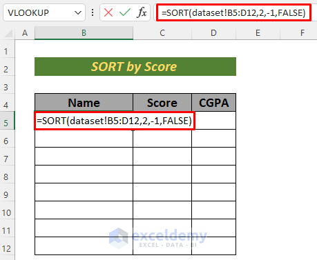

- Explanation:
  - We sort the students based on their obtained scores.
  - The array part of the SORT function is B5:D12 from the dataset sheet.
  - Set the sort_index to 2 (since scores are in the 2nd column).
  - Use -1 for descending order (top scores get higher rank).
  - Choose FALSE for an exact match.

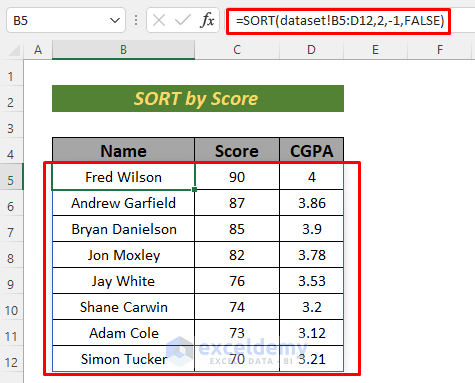
- Press ENTER to see the order of the students based on their scores.

Assign Ranks:
- Create a new column called Rank.
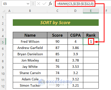
- In cell E5, enter this formula:

=RANK(C5,$C$5:$C$12,0)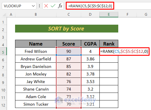

- Explanation:
  - The RANK function checks the value in cell C5 against the range C5:C12.
  - Absolute cell references ensure a fixed range.
  - A descending order 0 means better scores get higher ranks.

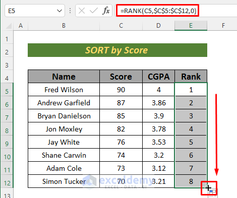
AutoFill:
- Press ENTER and use the Fill Handle to AutoFill the remaining cells.

Read More: How to Rank with Ties in Excel

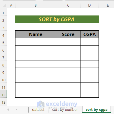
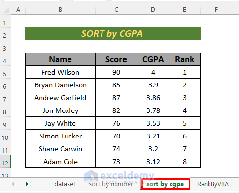
Method 2 – Using SORT and RANK Functions to Rank by CGPA

Set Up Your Sheet:
- Create a new sheet with columns for Names, Scores, and CGPAs.

Sorting with SORT Function:
- In cell B5, enter the following formula:

=SORT(dataset!B5:D12,3,-1,FALSE)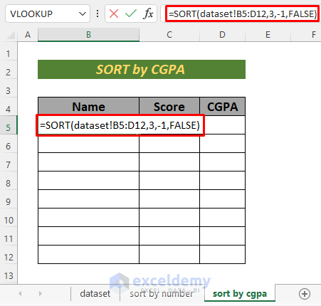

- Explanation:
  - We sort the students based on their current CGPA.
  - The array part of the SORT function is B5:D12 from the dataset sheet.
  - Set the sort_index to 3 (since CGPAs are in the 3rd column).
  - Use -1 for descending order (top CGPAs get higher ranks).
  - Choose FALSE for an exact match.

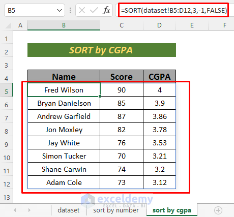
- Press ENTER button to see the students sorted by their CGPAs.

Assign Ranks:
- Create a new column called Rank.
- In cell E5, enter this formula:

=RANK(D5,$D$5:$D$12,0)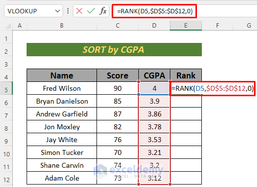

- Explanation:
  - The RANK function checks the value in cell D5 against the range D5:D12.
  - Absolute cell references ensure a fixed range.
  - A descending order 0 means better CGPAs get higher ranks.

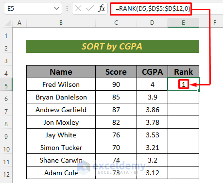
AutoFill:
- Press ENTER and use the Fill Handle to AutoFill the remaining cells.

Read More: Rank IF Formula in Excel

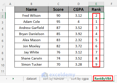
Method 3 – Ranking Data in Excel Using VBA and Sorting

In this method, we’ll leverage Microsoft Visual Basic for Applications (VBA) to rank data by scores. We won’t need the CGPA column for this ranking. Let’s walk through the procedure step by step:

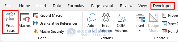
Open Visual Basic:
- Go to the Developer tab and open Visual Basic.

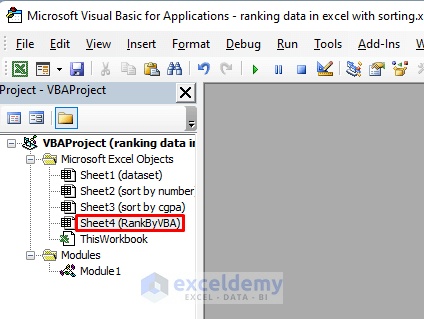
Access the VBA Window:
- The VBA window will appear.
- Open the sheet module where you want to run the VBA code.

Enter the VBA Code:
- Enter the following code in the module:

Private Sub Worksheet_Activate()
Dim last_row As Long
last_row = ActiveSheet.Cells(1, 1).CurrentRegion.Rows.Count
Range("B2:D" & last_row).Select
    Selection.AutoFilter
ActiveWorkbook.Worksheets("RankByVBA").AutoFilter.Sort.SortFields.Clear
   ActiveWorkbook.Worksheets("RankByVBA").AutoFilter.Sort.SortFields.Add Key:=Range("C2"), _
    SortOn:=xlSortOnValues, Order:=xlDescending, DataOption:=xlSortNormal
    With ActiveWorkbook.Worksheets("RankByVBA").AutoFilter.Sort
        .Header = xlYes
        .MatchCase = False
        .Orientation = xlTopToBottom
        .SortMethod = xlPinYin
        .Apply
    End With
     Selection.AutoFilter
    Range("E2").Select
    ActiveCell.Formula = "=RANK(C2,C:C,0)"
    Range("E2").Select
    Selection.AutoFill Destination:=Range("E2:E" & last_row), Type:=xlFillnormal
    Range("E2:E" & last_row).Select
     Range("E2").Select
End Sub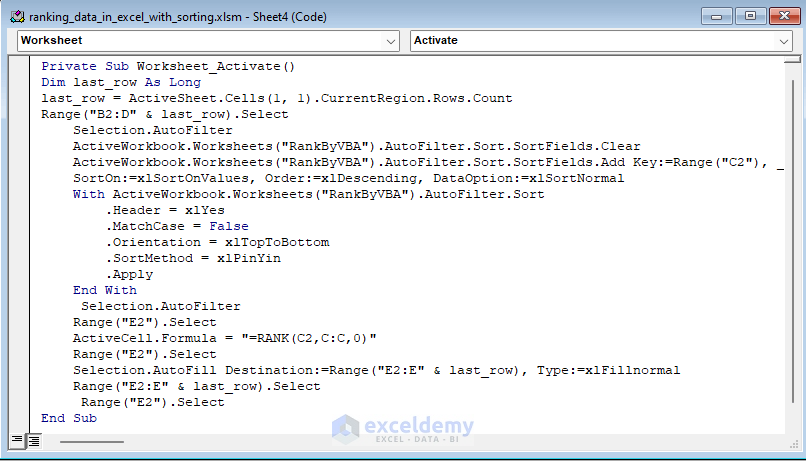

- Explanation:
  - We define a private worksheet and declare last_row as a Long variable.
  - Set the range to B2:D based on the Range method.
  - The working sheet is named RankByVBA, so we activate it using ActiveWorkbook.Worksheets(“RankByVBA”).
  - Apply AutoFilter, Sort, and SortFields properties.
  - Use the RANK formula to determine student ranks (column E).
  - Set column E as the destination range for the ranks.

Save and Return to Excel:
- Press CTRL + S to save the VBA code.
- Go back to your Excel sheet.

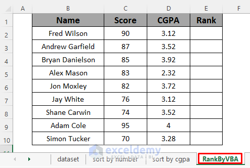
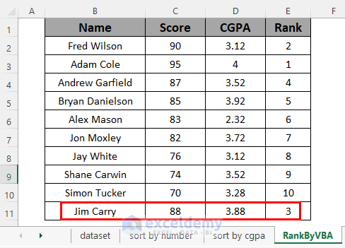
Observe Automatic Ranking:
- Switch to another sheet.

- Return to the RankByVBA sheet to see the students’ ranks automatically updated.

- Any new entries in the dataset will also receive their ranks automatically.

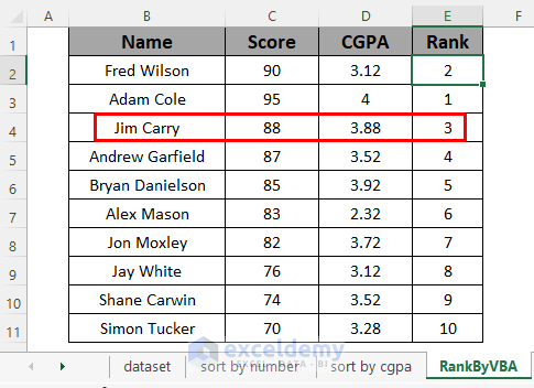
Verify Sorting:
- Move to another sheet and return to the RankByVBA sheet.
- Observe how the rank of the new entry is sorted in the dataset.