Method 1 – Using Conditional Formatting to Calculate and Highlight the Top 10 Percent of Values
Steps:
- Here’s a dataset of salespersons with their ID, Name, and Sales. We will calculate and highlight the top 10% of sales from the given dataset.
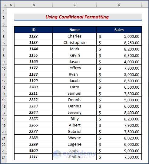
- Select the sales that you want to format.
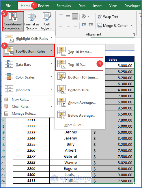
- Go to the Home tab.
- Click on Conditional Formatting under the Home tab.
- Choose the Top/Bottom Rules command.
- Click on the Top 10 % option.
- A pop-up window will be opened. Select the percentage option as you need. There is a list of colors. Choose your colors as per your need
- Press OK.

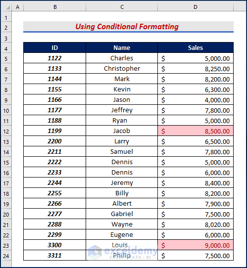
- You will see how the format of the sales column will be changed in the below image.
Read More: Ranking Data in Excel with Sorting
Method 2 – Calculate the Top 10 percent of Values by Utilizing PERCENTILE.EXC Function
Syntax
=PERCENTILE (array, k)Arguments Explanation
| Argument | Required or Optional | Value |
|---|---|---|
| array | Required | Pass the data values. |
| k | Required | Pass the number that will be representing the kth percentile. |
Steps:
- Select the E5 cell.
- Enter the following formula:
=D5>=PERCENTILE.EXC($D$5:$D$24,0.9)- Press Enter.

Formula Breakdown
- EXC($D$5:$D$24,0.9) here $D$5:$D$24 is the array where we will find the data. 0.9 is used as we want to get the top 10%.
- =D5> With this, we are comparing the top 10% percent with the data of the previous column.
- You will see the result for cell E5.
- Use the Fill Handle tool and drag it down from cell E5 to cell E24.

- You will get all the results in the below image.

- Select the entire data set.
- If you want to filter the data, click on the Filter icon under the Data tab.

- Click on the Top 10% Filter icon.

- Click on the Top 10% column and select only True.
- Press OK.

- You can see only the top 10% of sales data here.

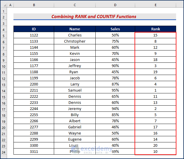
Method 3 – Combining RANK and COUNTIF Functions to Calculate Top 10 Percent of Values
Steps:
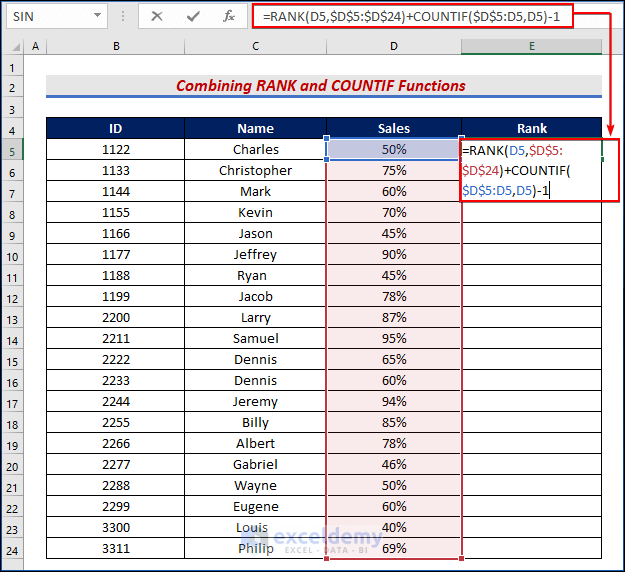
- Choose cell E5.
- Enter the following formula:
=RANK(D5,$D$5:$D$24)+COUNTIF($D$5:D5,D5)-1- Press Enter.
Formula Breakdown
- RANK(D5,$D$5:$D$24) will return the rank of each sales percentage.
- COUNTIF($D$5:D5, D5)-1 Here, the COUNTIF function will return the total count from the given dataset.
- You will see the Rank for cell E5.
- Use the Fill Handle tool and drag it down from cell E5 to cell E24.

- You will find all the ranks in the image below.
Read More: Excel Formula to Rank with Duplicates
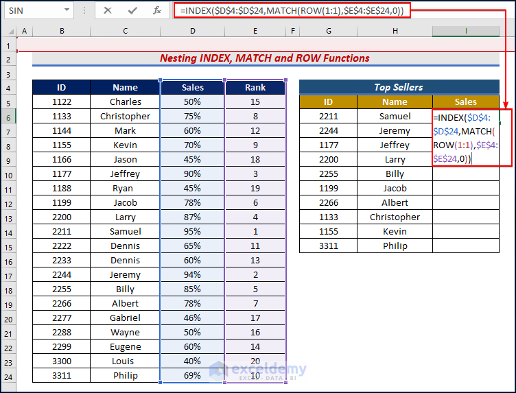
Method 4 – Nesting INDEX, MATCH and ROW Functions to Show All the Data of the Top 10 Percent of Values
Steps:
- Choose cell I6.
- Enter the following formula:
=INDEX($D$4:$D$24,MATCH(ROW(1:1),$E$4:$E$24,0))- Press Enter.
Formula Breakdown
- MATCH(ROW(1:1),$E$4:$E$24,0) this part will match the rows with the rank data and as we have declared 0 as the third argument, it will consider an exact match.
- Lastly, the INDEX function will figure out the data of the matched cell.
- You will see the sales for cell I6.
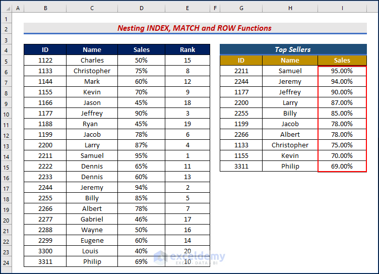
- Use the Fill Handle tool and drag it down from cell I6 to cell I15.

- You will find all the sales in the image below.
Read More: Ranking Based on Multiple Criteria in Excel
Things to Remember
- In the PERCENTILE function, k can be provided as a decimal (.7) or a percentage (70%)
- Also, the k must be between 0 and 1. Otherwise, PERCENTILE will return the #NUM! Error.
Download the Practice Workbook
Download the following Excel workbook to practice.
Related Articles
- Rank Within Group in Excel
- How to Rank with Ties in Excel
- How to Rank in Excel Highest to Lowest
- Rank IF Formula in Excel
<< Go Back to Excel RANK Function | Excel Functions | Learn Excel
Get FREE Advanced Excel Exercises with Solutions!
