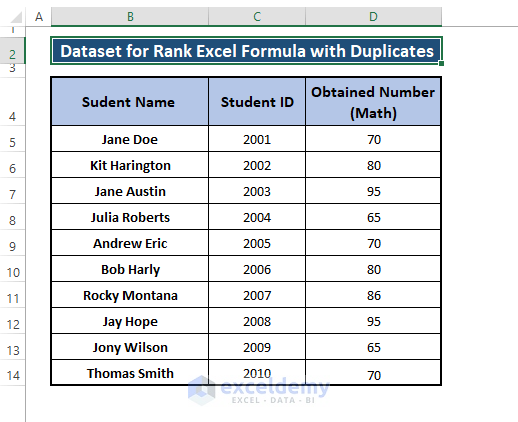
This is the sample dataset.
Method 1 – Ranking Duplicates by Using the RANK and COUNTIF Functions
The syntax of the RANK function is:
RANK(number,ref,[order])number; the rank whose number you want to find
ref; array, list, or range of numbers
[order]); a number that shows how to rank the numbe. [Optional]
0 – or default rank numbers in descending order
1 – rank numbers in ascending order
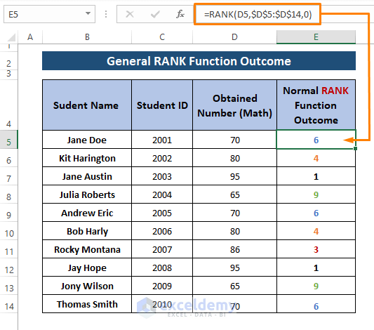
- Use the following formula to rank the numbers in the dataset:
=RANK(D5,$D$5:$D$14,0)D5=number
$D$5:$D$14=ref
0=descending order
This is the output.
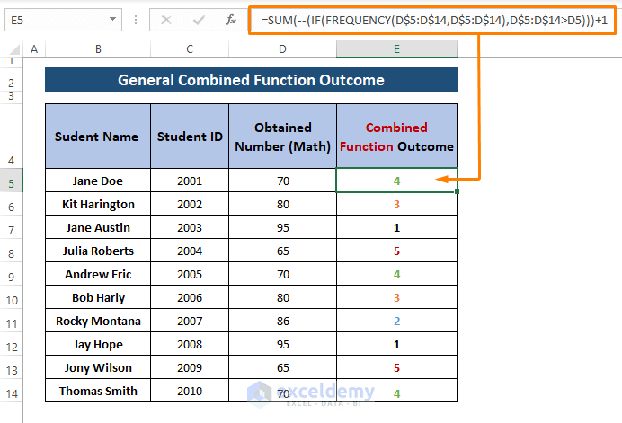
Slightly different rank types using a combination of functions can also be used:
=SUM(--(IF(FREQUENCY(D$5:D$14,D$5:D$14),D$5:D$14>D5)))+1The FREQUENCY, IF, and SUM functions were used. The formula ranks the duplicate values with the same rank number, displaying all other numbers.
1.1. In Descending Order
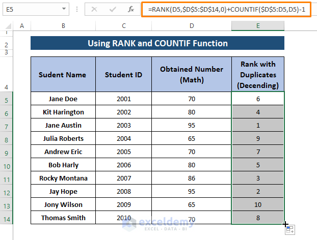
- To rank duplicates along with other values, enter the formula in a blank cell (E5)
=RANK(D5,$D$5:$D$14,0)+COUNTIF($D$5:D5,D5)-1The RANK function has all its arguments. The COUNTIF function has a range ($D$5:D5), and criteria (D5). 1 is subtracted from the COUNTIF result to ensure the ranking begins with 1. Otherwise, the formula returns rankings without rank 1.
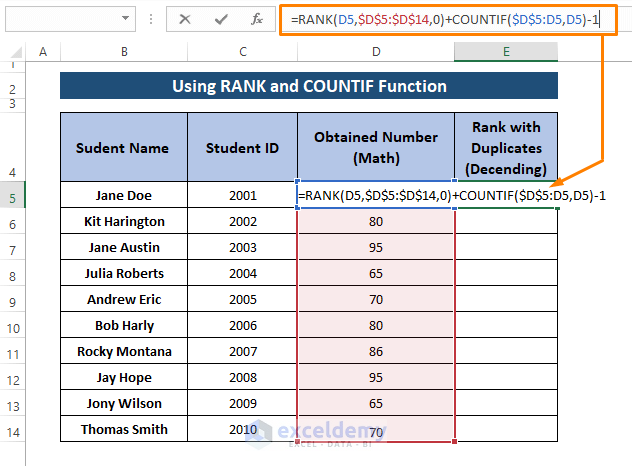
- Press ENTER and Drag the Fill Handle to display the ranks in descending order.
1.2. In Ascending Order
- Enter the formula below in a blank cell (E5).
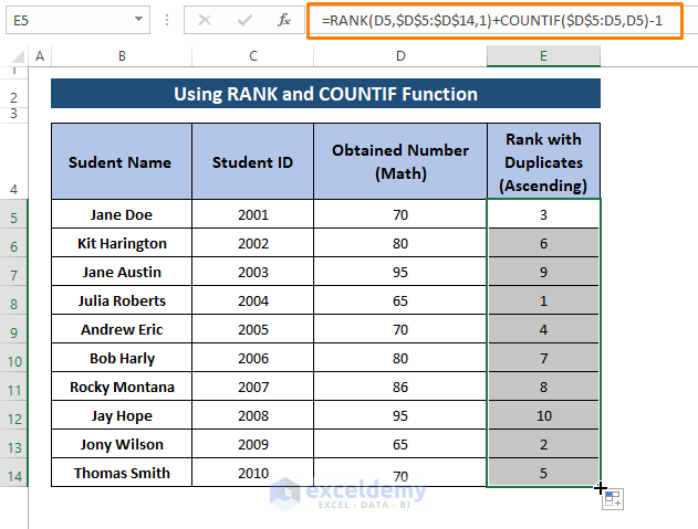
=RANK(D5,$D$5:$D$14,1)+COUNTIF($D$5:D5,D5)-1All the arguments in the formula return the same values as in 1.1. Descending Order .
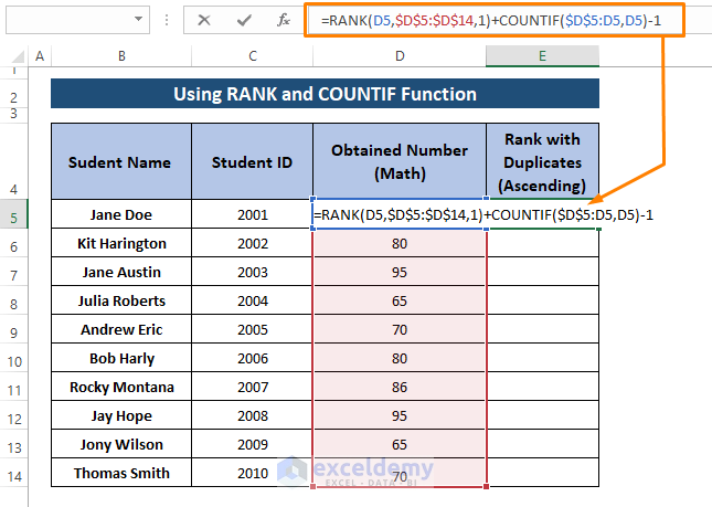
- Press ENTER and Drag the Fill Handle to see the ranks in ascending order.
Method 2 – Combining the RANK and COUNTIFS Functions (with Criteria)
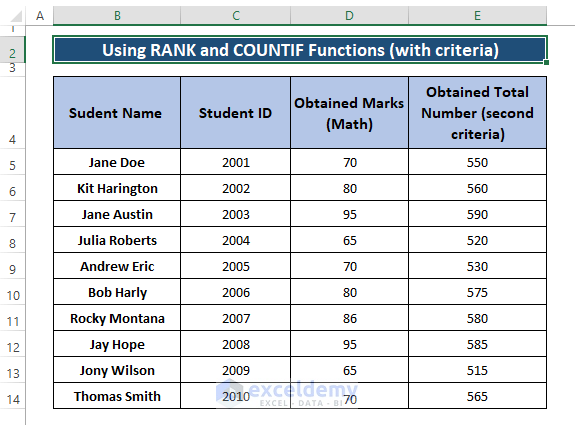
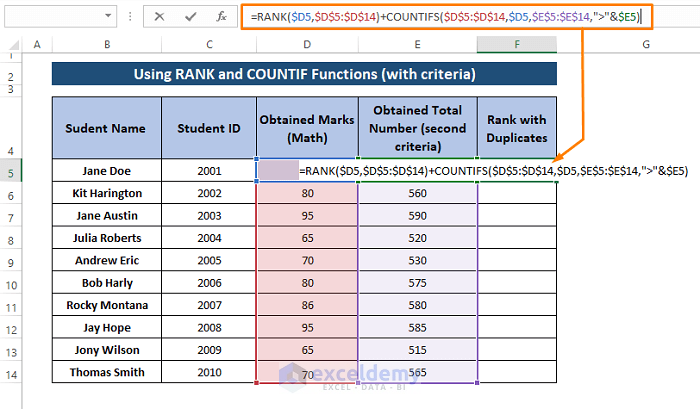
This is the sample dataset.
Step 1:
- Enter the following formula in a blank cell (F5).
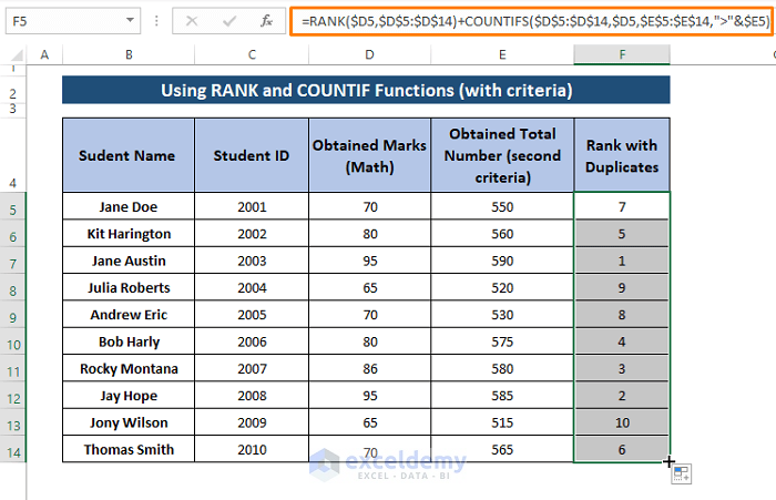
=RANK($D5,$D$5:$D$14)+COUNTIFS($D$5:$D$14,$D5,$E$5:$E$14,">"&$E5)An additional criterion is added through the COUNTIFS function. It assigns the total number range ($E$5:$E$14) greater than the first entry ($E5). The formula compares all the entries and ranks them.
Step 2:
- Press ENTER and drag the Fill Handle.
This is the output.
Read More: How to Rank Within Group in Excel
Method 3 – Merging the IF, RANK and COUNTIF Functions
The syntax of the IF function is:
=IF (logical_test, [value_if_true], [value_if_false])This is the formula:
=IF($D5="","",RANK($D5,$D$5:$D$14,0)+COUNTIF($D$5:$D5,$D5)-1)$D5=””, is the logical_test. If the test returns TRUE, the formula inserts a blank in cell (E5). Otherwise, the RANK($D5,$D$5:$D$14,0)+COUNTIF($D$5:$D5,$D5)-1 portion of the formula displays the rank. The [value_if_false] formula portion defines all arguments.
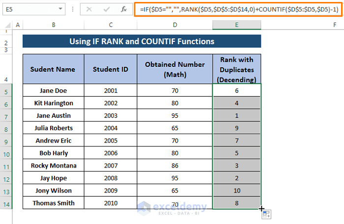
3.1. In Descending Order
- Enter the following formula in any blank cell (E5).
=IF($D5="","",RANK($D5,$D$5:$D$14,0)+COUNTIF($D$5:$D5,$D5)-1)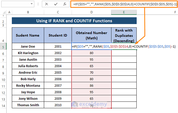
- Press ENTER and drag the Fill Handle to see the output.
3.2. In Ascending Order
- Enter this formula in a blank cell (E5).
=IF($D5="","",RANK($D5,$D$5:$D$14,1)+COUNTIF($D$5:$D5,$D5)-1)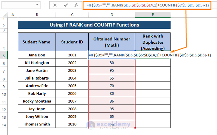
- Press ENTER.
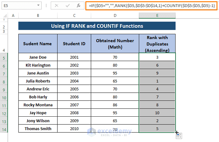
- Drag the Fill Handle to rank all entries in the dataset.
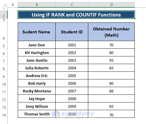
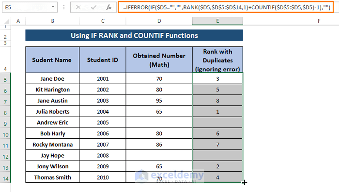
The following dataset contains blank entries. A formula can ignore them and return the ranks.
- Modify the IF, RANK, and COUNTIF formula as below and enter it in a blank cell (E5)
=IFERROR(RANK($D7,$D$5:$D$14,1)+COUNTIF($D$5:$D7,$D7)-1,"")The IFERROR formula displays blank cells in entries where empty cells are referred to, otherwise inserts the ranks.
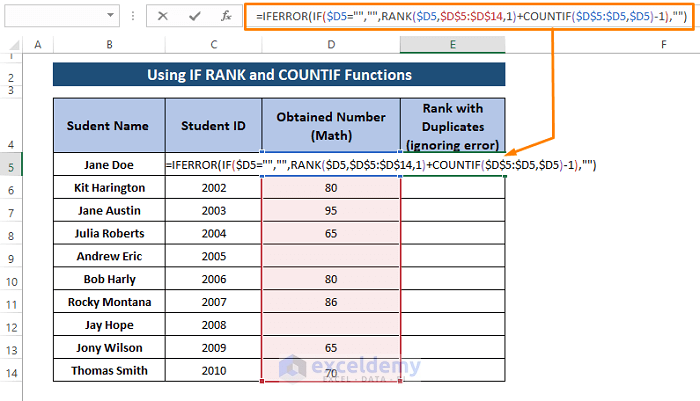
- Press ENTER and drag the Fill Handle to see all the ranks.
Read More: Ranking Data in Excel with Sorting
Download Excel Workbook
Related Articles
- How to Rank with Ties in Excel
- Rank IF Formula in Excel
- How to Rank in Excel Highest to Lowest
- How to Calculate Top 10 Percent in Excel
- Ranking Based on Multiple Criteria in Excel
<< Go Back to Excel RANK Function | Excel Functions | Learn Excel
Get FREE Advanced Excel Exercises with Solutions!


Rank in excel
I think it injustice if 3 students obtained same marts and 3 different ranks.
If ranks same then the next two ranks are absent
Hello Jamil Khan,
Thank you for your question. Actually, this is how the RANK function works, that is to say, it ranks the duplicate values in ascending or descending order according to the given argument. Now, to have the same ranks for identical values you can follow Method 1 or download the Excel file that the ExcelDemy team has created.
Download the Excel File below.
Ranking Duplicates.xlsx
I want to use the data that is ranked for a related purpose. e.g.
Competition marks: two competitors with same result (first or Rank 1)’
The ID for those two would be used for other purpose but I cannot find a formula to identify them separately and return their ID for another function. I have used =INDEX(X5:X30,MATCH(3,W5:W30,0))but it only works with one (the first in the list) of the RANK 1 results – it does not identify the second.
Hello Phil,
You can use the FILTER function (for Excel 365/2021) or a combination of INDEX and SMALL to retrieve multiple IDs corresponding to the same rank.
Try this formula if you’re using Excel 365/2021:
=FILTER(X5:X30, W5:W30=3)
This will return all IDs where the rank is 3.
If you’re using an older version of Excel, use this array formula:
=INDEX(X$5:X$30, SMALL(IF(W$5:W$30=3, ROW(W$5:W$30)-ROW(W$5)+1), ROW(A1)))
1. Press Ctrl + Shift + Enter after typing the formula (if using older Excel).
2. Drag it down to get multiple results.
Let me know if you need further clarification!
Regards
ExcelDemy