Basics of FREQUENCY Function: Summary & Syntax
Summary
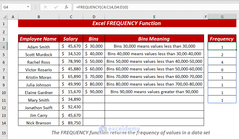
The Excel FREQUENCY function returns how often numeric values occurred within the ranges you specify in a bin table of a set of data or dataset. It will calculate and return a frequency distribution. This function returns the distribution as a vertical array of numbers that represent a count per bin. Remember one thing, the FREQUENCY function always returns an array with one more item than bins in the bins_array. This is designed to catch any values greater than the largest value in the bins_array.
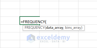
Syntax
FREQUENCY (data_array, bins_array)
Arguments
| Arguments | Required/Optional | Explanation |
|---|---|---|
| data_array | Required | It is an array of values for which you want to get frequencies. |
| bins_array | Required | It is an array of intervals for grouping values. The interval is also known as “bins”. |
Return Value
The FREQUENCY function returns the frequency of values in a data set.
Example 1 – Using The FREQUENCY Function to Get Often Occurred Values
To illustrate, let’s try to get the often-occurred values from the Salary column.
⏩ In cell F4, enter the following formula:
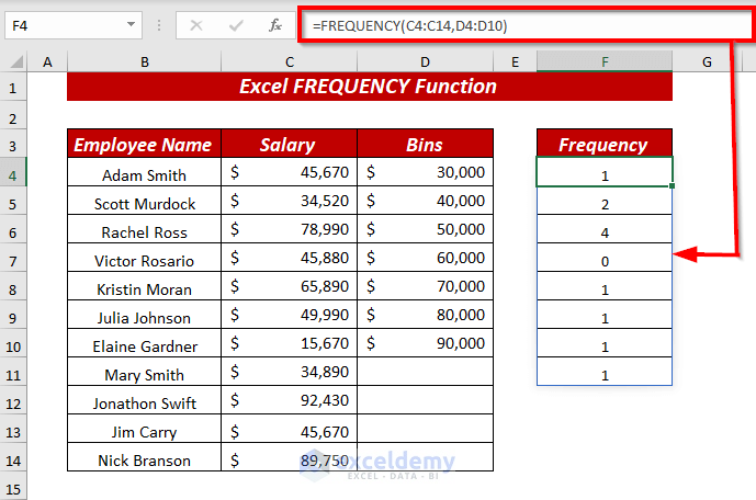
=FREQUENCY(C4:C14,D4:D10)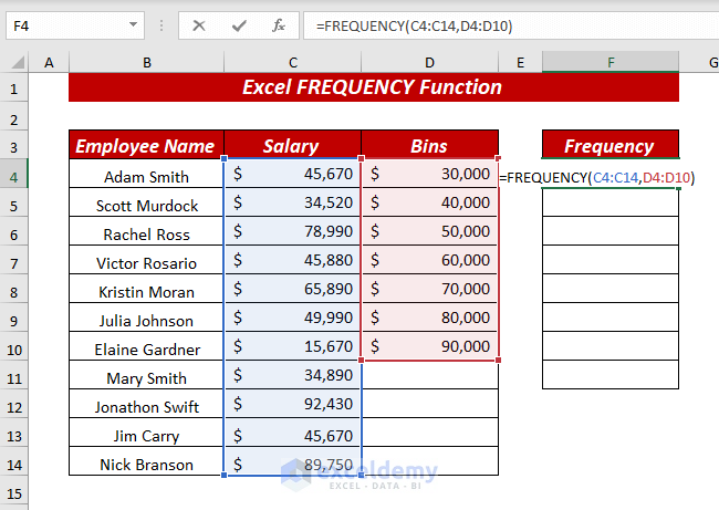
I selected the range C4:C14 as data_array and the range D4:D10 as bins_array.
Press ENTER. It will return the frequently occurring values from the selected range.
Example 2 – Using The FREQUENCY Function to Figure Out Frequency Percentages
⏩ In cell F4, enter the following formula:
=FREQUENCY(C4:C14,D4:D10)/COUNT(C4:C14)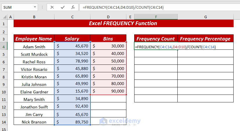
The range C4:C14 is the data_array and range D4:D10 is bins_array.
In the COUNT function, range C4:C14 is value1.
Divide the frequently occurring values by the count of the selected range.
Press ENTER, and the FREQUENCY function will return the result.
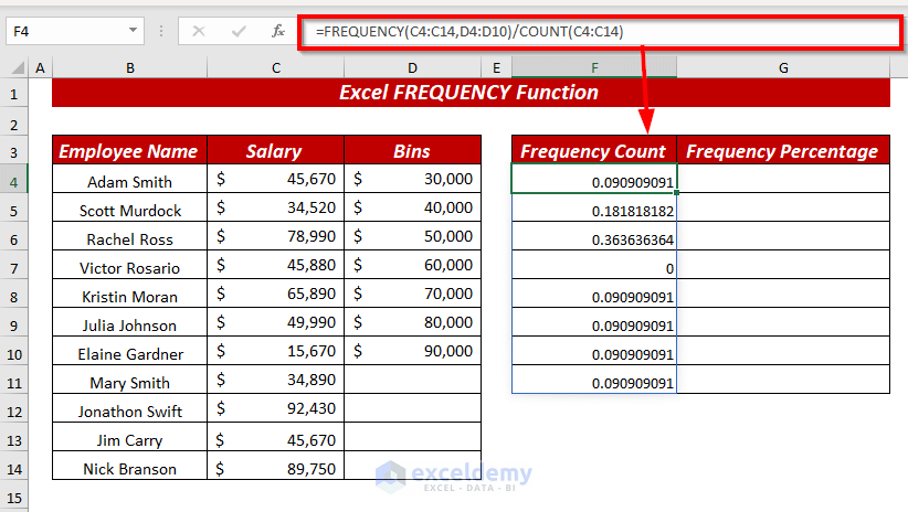
To convert the result into a percentage,
Select the cell range (G4:G11)
Open the Home tab >> from Number group >> select %.
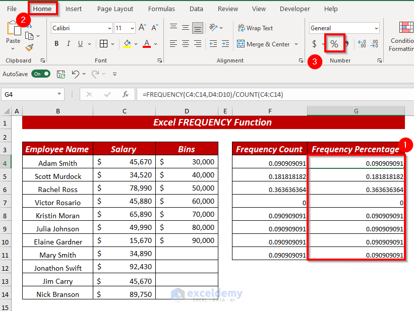
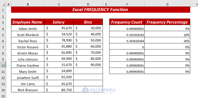
The result will be converted into percentages.
Example 3 – Using Excel FREQUENCY & SUM Function with Operator
⏩ In cell E4, enter the following formula:
=SUM(--(FREQUENCY(B4:B14, B4:B14) >0))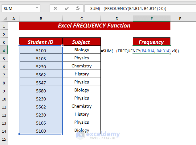
I used FREQUENCY(B4:B14, B4:B14) >0) as number1.
Range B4:B14, B4:B14 is the data_array, and range B4:B14, B4:B14 is the bins_array. >0 is used to get the values occurring frequently.
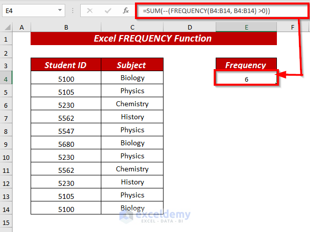
The SUM function will sum up the frequently occurring students’ IDs.
(–) is used to get the result in binary form.
Press ENTER to will return the sum of frequently occurred Student IDs.
Example 4 – Using Excel TRANSPOSE & FREQUENCY Function to Get Horizontal Array of Results
⏩ In cell F4, enter the following formula:
TRANSPOSE(FREQUENCY(C4:C14,D4:D10))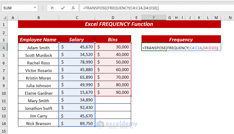
In the TRANSPOSE function, FREQUENCY(C4:C14,D4:D10) as an array.
In the FREQUENCY function, range C4:C14 is the data_array, and range D4:D10 is the bins_array.
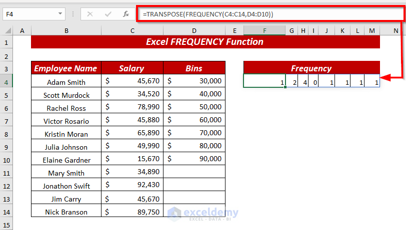
The FREQUENCY function will return the results vertically and the TRANSPOSE function will transpose it horizontally.
Press ENTER, and you will get the results in a horizontal array.
Example 5 – Using Excel FREQUENCY Function to Count Unique Values in A Range with Criteria
⏩ In cell F4, enter the following formula:
=SUM(--(FREQUENCY(IF(C4:C14=F4,MATCH(B4:B14,B4:B14,0)),ROW(B4:B14)-ROW(B4)+1)>0))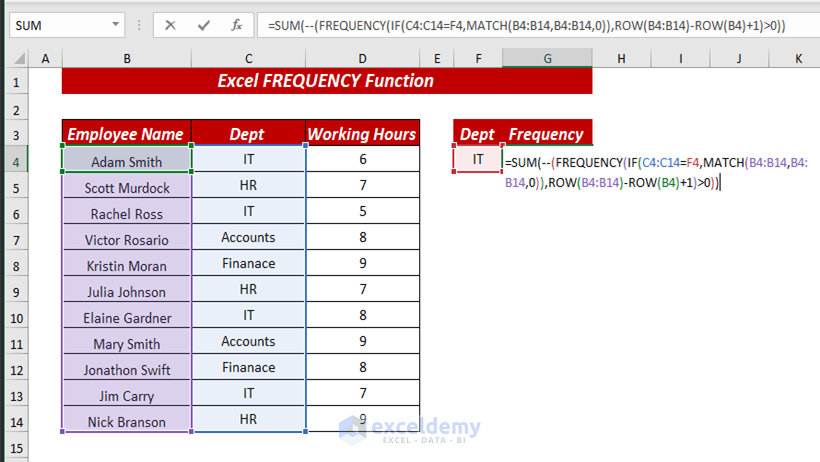
In the SUM function, FREQUENCY(IF(C4:C14=F4,MATCH(B4:B14,B4:B14,0)),ROW(B4:B14)-ROW(B4)+1)>0 is used as number1.
In the FREQUENCY function, IF(C4:C14=F4,MATCH(B4:B14,B4:B14,0)) is the data_array, and ROW(B4:B14)-ROW(B4)+1) is bins_array. And used greater than >0.
In the IF function, C4:C14=F4 is used as logical_test, and MATCH(B4:B14,B4:B14,0) as value_if_true.
In the MATCH function, range B4:B14 is the lookup_value, range B4:B14 is the lookup_array and 0 is the match_type.
Multiple ROW functions are used. In the first ROW function, range B4:B14 is used as a reference. In the second ROW function, cell B4 is used as a reference. And 1 is added with the cell reference.
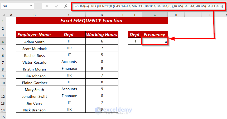
Press ENTER, and you will get the count of frequently occurring unique values in a range while applying criteria.
Example 6 – Find Frequent Values for Time
⏩ In cell F4, enter the following formula:
=FREQUENCY(D4:D14,E4:E8)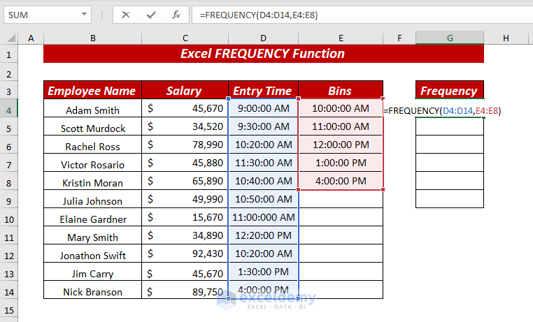
In the FREQUENCY function, range D4:D14 is the data_array, and range E4:E8 is the bins_array.
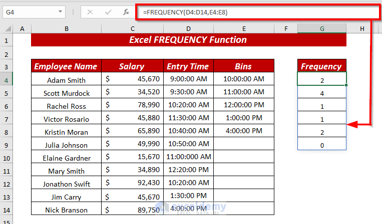
Press ENTER, and the FREQUENCY function will return the frequently occurring times from the selected range.
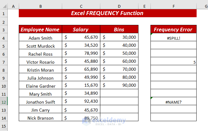
Things to Remember
The FREQUENCY function will show the #NAME error if you misspell the function name.
The FREQUENCY function will show the #SPILL error if one or more cells in the spill range are not completely blank.
Download to Practice
<< Go Back to Excel Functions | Learn Excel
Get FREE Advanced Excel Exercises with Solutions!
